2026-06-29 20:12:05
The calculator utility bc has a minimal math library. For example, there’s no tangent function because you’re expected take the ratio of sine and cosine. (The Gnu version of bc does have a function for tangent, but the POSIX version does not.) And yet bc includes support for Bessel functions J(x).
The bc function j takes two arguments. Is the first argument n or x? Grok said the function arguments are j(n,x). I thought I should run man bc just to make sure, and it said
j(x, n) Returns the bessel integer order n (truncated) of x.
So Grok says j(n,x) and the documentation that ships with the software says j(x,n). Which one should you believe? Neither! You should run a little test.
~$ bc -l
>>> j(1, 0)
0
>>> j(0, 1)
.76519768655796655144
Now J1(0) = 0, so apparently the first argument is the order n. Grok was right and the man page was wrong.

As further confirmation, let’s see which argument is truncated.
>>> j(1.2, 3.4)
.17922585168150711099
>>> j(1, 3.4)
.17922585168150711099
>>> j(1.2, 3)
.33905895852593645892
The first argument is truncated to an integer value, so that’s the order n.
Turns out there’s a bug in the man page. The man page text above comes from running man bc on my Macbook. On my Linux box, the documentation is correct. It says
j(n,x) The Bessel function of integer order n of x.
The software produces the same results on both computers. It’s just a documentation bug.
The version running on my Macbook is the version that ships with the OS. It’s not the Gnu version, though the documentation says “This bc is compatible with both the GNU bc and the POSIX bc spec.” It has a function t for tangent, for example, which a POSIX version does not. But if you run bc --standard -l attempting to call t produces an error.
2026-06-28 08:33:33
Here’s a crazy bash one-liner I found via an article by Peter Krumins:
echo {w,t,}h{e{n{,ce{,forth}},re{,in,fore,with{,al}}},ither,at}
This prints 30 English words:
when, whence, whenceforth, where, wherein, wherefore, wherewith, wherewithal, whither, what, then, thence, thenceforth, there, therein, therefore, therewith, therewithal, thither, that, hen, hence, henceforth, here, herein, herefore, herewith, herewithal, hither, hat
This post will explain how the one-liner works.
Bash brace expansion iterates through all possibilities listed within curly braces, with possibilities separated by a comma. Note that the comma is a separator and not a terminator. And so, for example, the expression {w,t,} is effectively {w,t,""}.
When bash sees two brace expressions, these expand to the cartesian product of the two expressions. For example,
echo {A,B}{1,2,3}
produces
A1 A2 A3 B1 B2 B3
In the expression above we have
{w,t,}h{e…,ither,at}
So the expansion will enumerate all possibilities of {w,h,} multiplied by all possibilities of {e…,ither,at} where e… is itself a brace expression.
A diagram will help a lot.
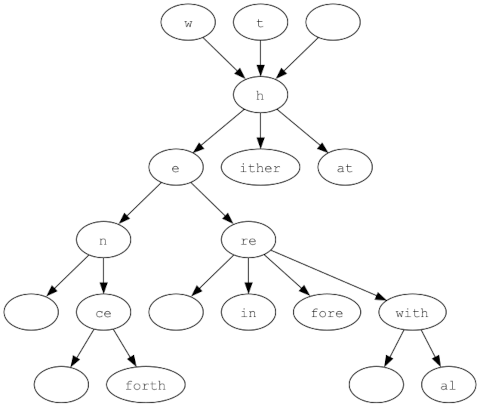
The brace expansion does a depth-first traversal of this tree.
The post Brace expansion tree first appeared on John D. Cook.2026-06-28 02:12:03
The previous post looked at how many digits are in the reduced fraction for the nth harmonic number. I was curious about how long the cycle of digits in a harmonic number might be.
I wrote about the period length for the digits of fractions almost a decade ago. This post includes code so I can apply it to harmonic denominators.
from sympy import lcm, factorint, n_order

def period(n):
    factors = factorint(n)
    exp2 = factors.get(2, 0)
    exp5 = factors.get(5, 0)
    r = max(exp2, exp5)

    d = n // (2**exp2 * 5**exp5)
    s = 1 if d == 1 else n_order(10, d)
    return (r, s)
This function returns two numbers: r is the number of non-repeating digits at the beginning and s is the length of the repeating part.
The following code
from functools import reduce

def lcm_range(n):
    return reduce(lcm, range(1, n + 1))

print( period( lcm_range(50) ) )
prints (5, 1275120) meaning that 1/lcm(1, 2, 3, …, 49, 50) has five non-repeating digits following by 1,275,120 digits that repeat ad infinitum. And so the decimals in the expansion of H50 have a cycle length of 1,275,120.
The post When will the decimals in a/b repeat? first appeared on John D. Cook.2026-06-27 20:51:42
The previous post looked at writing the harmonic numbers as reduced fractions and estimating the number of digits in the numerator and denominator based on asymptotics. This is a follow up post with plots.
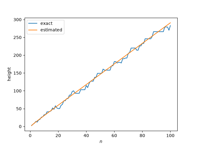
We’ll choose our base b to be 2. And we’ll look at the total number of bits in both the numerator and denominator, which we will use as the height of the fractions.
First, let’s look at the actual and estimated heights, using the estimates from the previous post.
Next let’s look at the difference between the actual and estimated heights.
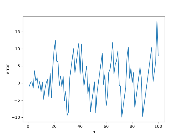
In the previous post I looked at n = 50, which was kind of a lucky choice, the error being smaller than usual. I had also looked at, but didn’t publish, n = 100, which would be an unlucky choice.
Finally, let’s look at the relative error in the estimates, and plot over a larger range of n.
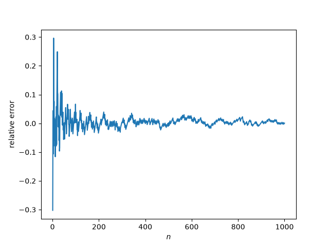
The error goes to zero, as predicted by the asymptotic estimates. And it goes noisily, which you’d expect since the heights are related to the distribution of primes.
The post Height of harmonic numbers first appeared on John D. Cook.2026-06-27 09:51:03
The nth harmonic number is the sum of the reciprocals of the first n positive integers.
Hn = 1 + 1/2 + 1/3 + 1/4 + … + 1/n
The product of all the denominators is n!, so you could write Hn as a fraction
Hn = p/q
where p = n! Hn is an integer and q = n!.
While p/q is a way to write Hn as a fraction, it’s not the most efficient because p and n! will have common factors.
If we write Hn as a reduced fraction, the denominator will be the least common multiple of the integers 1 through n. That number is asymptotically exp(n). That estimate follows from the prime number theorem.
So for large n the denominator will be roughly exp(n), and in base b it would have around
n/log(b)
digits.
The numerator will be exp(n) Hn, and since Hn is asymptotically log(n) + γ, the numerator for large n will be roughly
exp(n) (log(n) + γ)
and will have around
(n + log log(n) ) / log(b)
digits.
Let’s see how well our asymptotic estimates work for n = 50. The 50th harmonic number is
H50 = 13943237577224054960759 / 3099044504245996706400.
This fraction has 23 digits in the numerator and 22 in the denominator. We would have predicted around
(50 + log(log(50)))/log(10) = 22.3
digits in the numerator and
50/log(10) = 21.7
digits in the denominator.
Let’s try a larger example, looking at the 1000th harmonic number in binary. We’ll use the following Python code.
from fractions import Fraction

def bits(n):
    H = sum(Fraction(i, i+1) for i in range(1, n+1))
    p, q = H.numerator, H.denominator
    # subtract 2 because bin returns a string starting with 0b.
    return len(bin(p)) - 2, len(bin(q)) - 2

print(bits(1000))
This returns 1448 and 1438. We would have estimated
(1000 + log(log(1000)))/log(2) = 1445.4
bits in the numerator and
1000/log(2) = 1442.7
bits in the denominator.
Update: See the next post for plots as a function of n.
2026-06-26 03:20:09
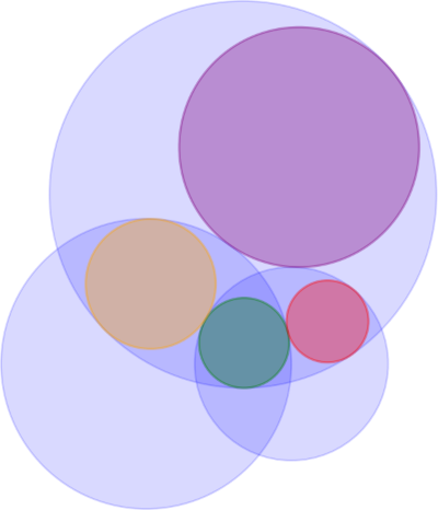
Hart’s theorem says
If a triangle be formed by the arcs of three circles, the inscribed and the three escribed circles are all tangent to a new circle or line.
Here “triangle” means a three-sided figure whose sides are portions of a circle. The inscribed circle is the largest circle that can fit inside the three-sided figure.
The “escribed” circles are analogous to the excircles in the previous post: you extend two sides and find a circle that is tangent to the triangle side and the extended side. The difference here being that the side extensions are now circles.