2026-06-04 23:16:14
![]()

Whether one’s dealing with biology, economics, politics or a host of other fields, it’s common to encounter situations that can be modeled as involving two agents that repeatedly compete with each other. One imagines that at each step each agent can take one of a certain set of actions, and that then—in a classic game theory way—each agent (or “player”) gets a certain fixed “payoff” based on the action they and their opponent take. But how do the agents decide what action to take? We imagine that each agent has a certain fixed procedure—or “strategy”—for making its decisions. And we imagine that the input to each of those decisions is the sequence of past actions that the agent and its opponent have taken.
There’s been lots of work done over the course of nearly a century on particular choices of strategies. But something I’ve long been curious about is what happens if one systematically considers all possible strategies. And if we think of strategies as programs this becomes a question to which we can immediately apply ruliological methods. Which is what I’m going to do here.
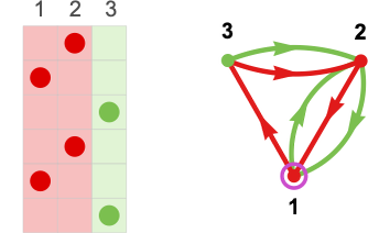
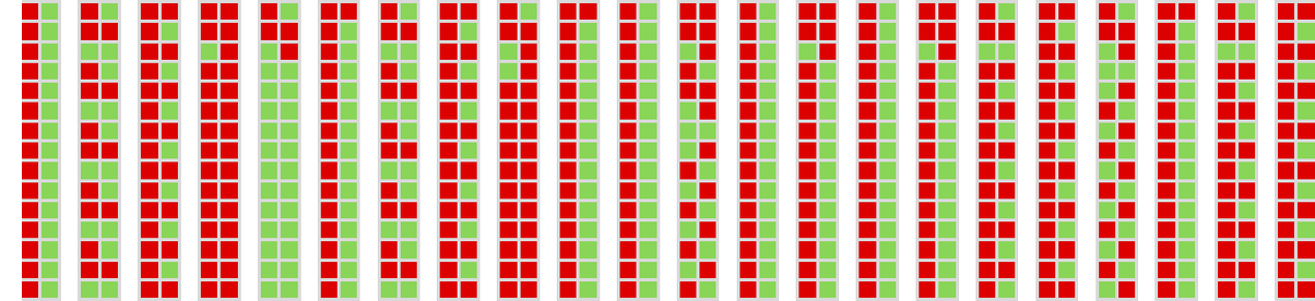
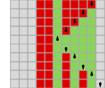
To be more specific about the setup, let’s assume that at each step, each agent takes one of two possible actions, indicated by ![]() and
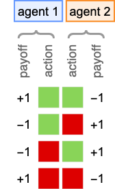
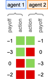
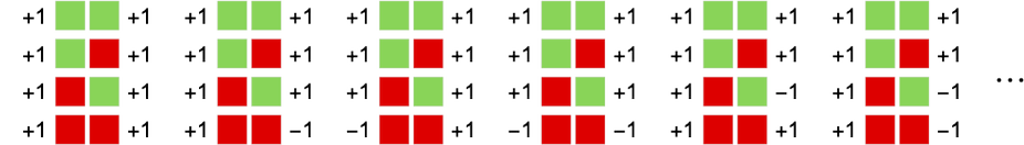
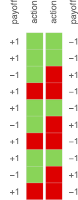
and ![]() . And for now let’s take the payoffs to be the ones for the classic “match-or-not” (“matching pennies”) game—in which player 1 has the bigger payoff when there’s a match, and player 2 has the bigger payoff when there isn’t a match:
. And for now let’s take the payoffs to be the ones for the classic “match-or-not” (“matching pennies”) game—in which player 1 has the bigger payoff when there’s a match, and player 2 has the bigger payoff when there isn’t a match:
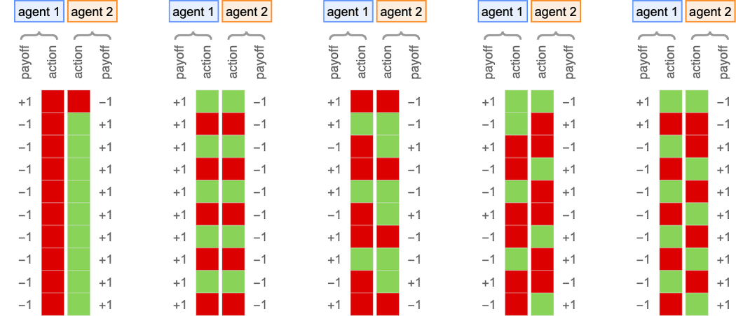
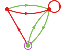
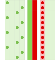
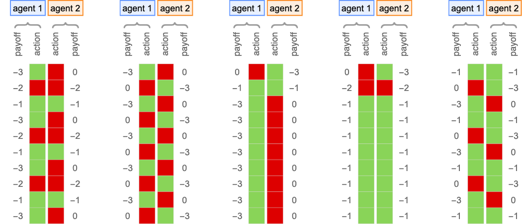
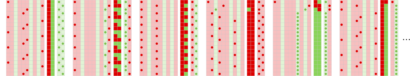
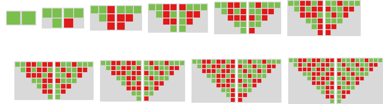
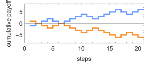
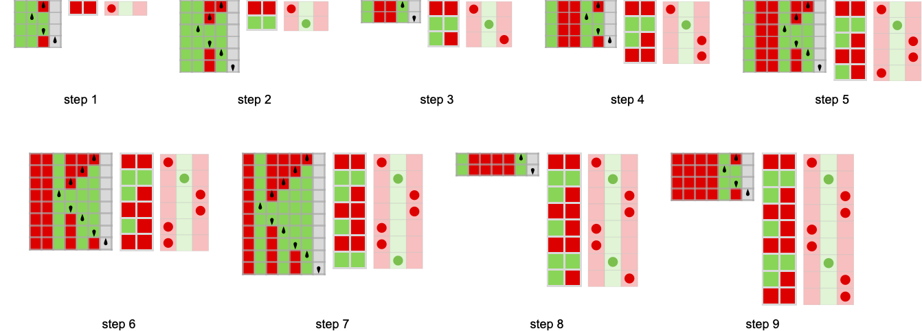
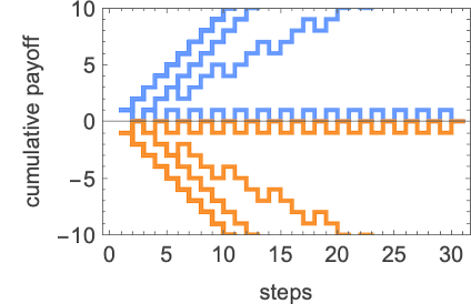
So what happens when agents repeatedly play this game? Well, it depends on their strategies. Here are a few examples for several different choices of each agent’s strategy:
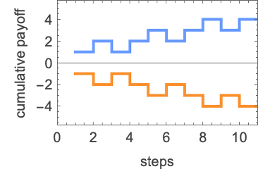
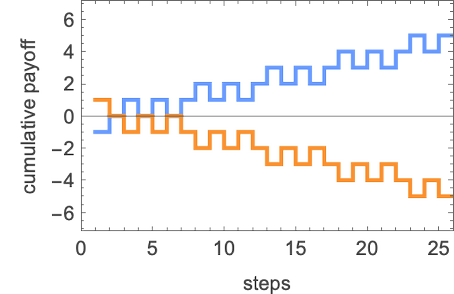
Plotting the cumulative payoffs for the two agents (represented by ![]() and
and ![]() ) in each of these cases we get:
) in each of these cases we get:
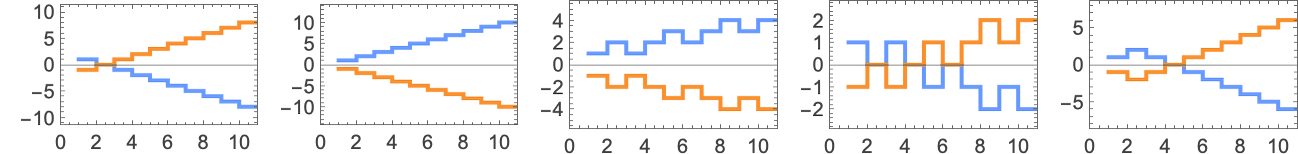
Often we’ll consider the “winning agent” to be the one that has the numerically largest cumulative payoff (i.e. is eventually on top in these plots) after a certain number of steps. And with a criterion like this, we’ll be able to rank different programs against each other—and in general explore the ruliology of competition.
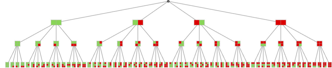
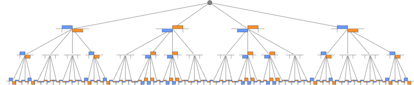
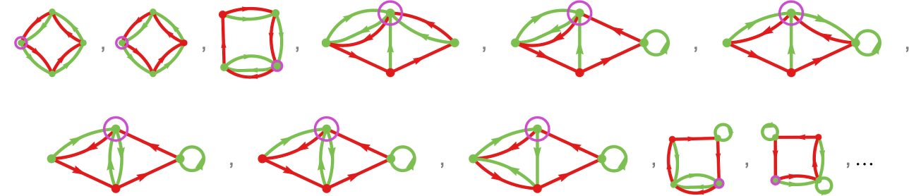
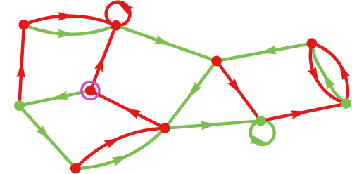
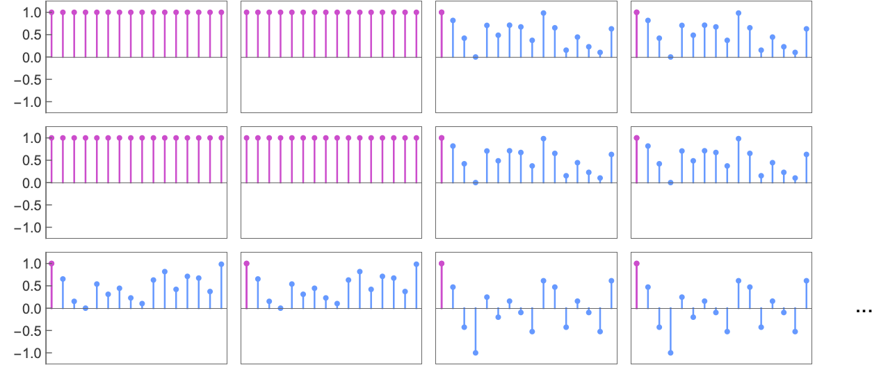
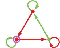
With the basic setup we’re using, we can represent all possible sequences of actions by a multiway graph:
For any given sequence of actions, there is then a cumulative payoff for each agent for our match-or-not game:
If each agent adopts a particular strategy, this will define a particular path through the multiway graph. For the strategies used in the examples above, the paths are:
What does it take to have a winning strategy? In what follows, we’ll consider strategies based on several different types of programs. But one basic question we can always ask is whether what turn out to be the winning strategies tend to be based on programs that are more complicated, or less so—or to show behavior that is more complicated, or less so.
In other words, if you want to win, should you typically be trying to build up something complicated? Or should you instead expect to be able to find a “simple hack” that will “crack the game” and—at least usually—let you win? In effect, we’re asking whether competition tends to lead to complexity, or simplicity.
I’ve recently looked at minimal models of both biological evolution and machine learning, in which one is adaptively evolving programs in order to maximize some externally imposed fitness function. And what I’ve found is that even when the fitness function one uses is simple, the behavior of the programs that maximize it is normally quite complex. In other words, adaptive evolution will tend to make even a simple, fixed objective be achieved in a complicated way.
So what if instead of having a fixed, externally imposed objective, our goal is just broadly to win against other agents? Does such—potentially open-ended—competition lead us to more complex behavior (or more complex programs), or not? That’s the kind of question we’re going to be able to explore here by looking at the ruliology of competition.
Finite state machines can be thought of as defining extremely simple programs (that might model pathways in biology, decision processes in economics, etc.). And to start our investigation of the ruliology of competition we’re going to look at strategies defined by finite state machines.
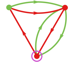
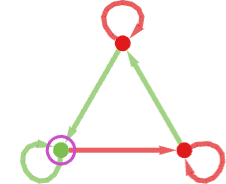
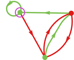
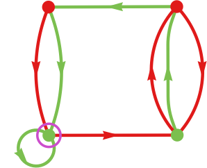
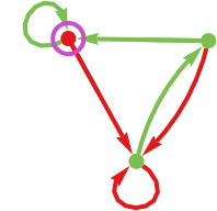
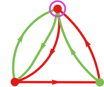
A typical example of a finite state machine (here with 3 states) is:
We’re going to use this finite state machine to define a strategy for an agent. To see how this works, let’s say that the sequence of actions taken by the agent’s opponent have been:
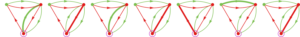
The idea is to use this sequence of actions to define a path in the finite-state-machine graph, then to determine the next action from the color of the state reached. We start at the vertex with the incoming arrow, then successively follow the edge whose color matches the next move made by the opponent:
At the end of this process we’ll reach some vertex in the graph (i.e. some state in the finite state machine). In the particular case shown here, the state we reach is ![]() . And then we take the output of the strategy—i.e. the next action for the agent to take—to be
. And then we take the output of the strategy—i.e. the next action for the agent to take—to be ![]() .
.
It’s sometimes convenient to show the states of the finite state machine arranged on a line:
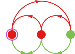
And then we can summarize the path taken with a certain input by showing the successive states reached:
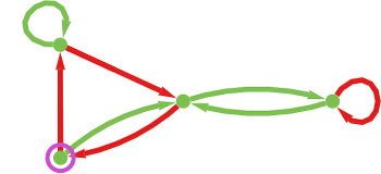
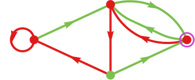
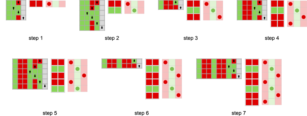
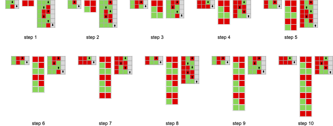
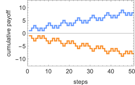
So what happens if two finite state machines compete? The basic idea is that the successive outputs from one machine become the successive inputs to the other, and vice versa. If our second machine is
then we can represent the behavior of the machines by:
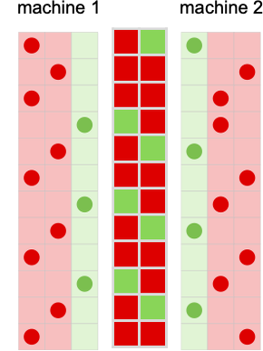
If the payoffs we use are for the match-or-not game, then their cumulative values for these machines are
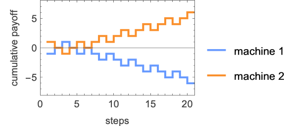
so that in the end agent 2 can be considered the winner.
It’s important to note here that in the setup we’re using, everything is deterministic: at every step, each agent takes an action that is deterministically computed using its strategy from the past history of moves. It’s a different setup from what’s most often studied in game theory, where each move is in effect considered independently, but where there can be probabilities for different actions (“mixed strategies”)—and where in the end averaging is done over “different possible rolls of the dice”.
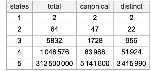
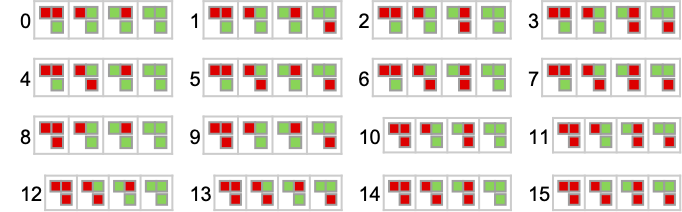
The number of possible graphs for finite state machines with s states is (2 s2)s. But some of those graphs correspond to machines with identical behavior—so that the number of distinct machines is smaller:
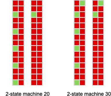
In the 2-state case, the 22 distinct machines are
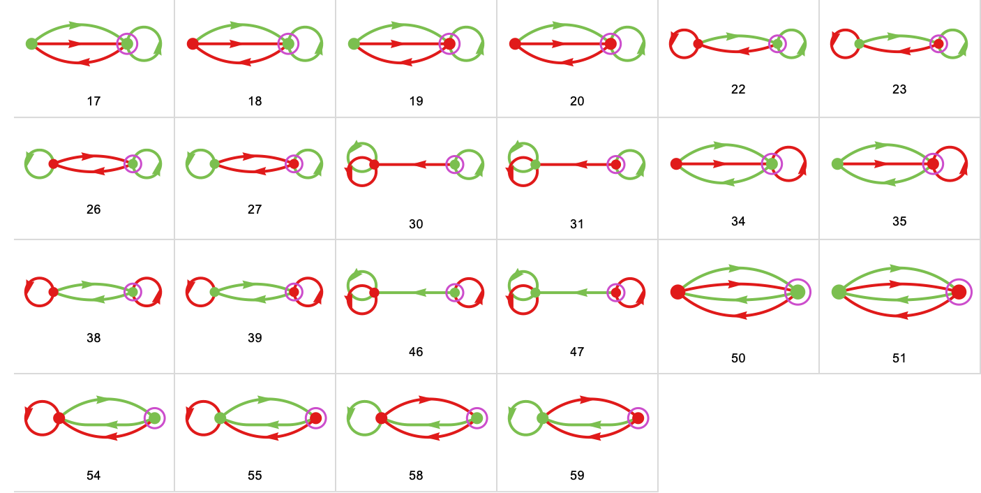
where we’ve identified each machine by a number.
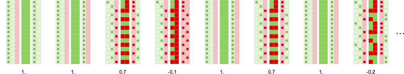
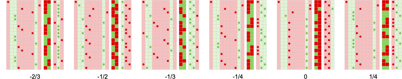
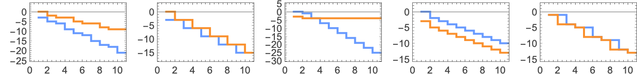
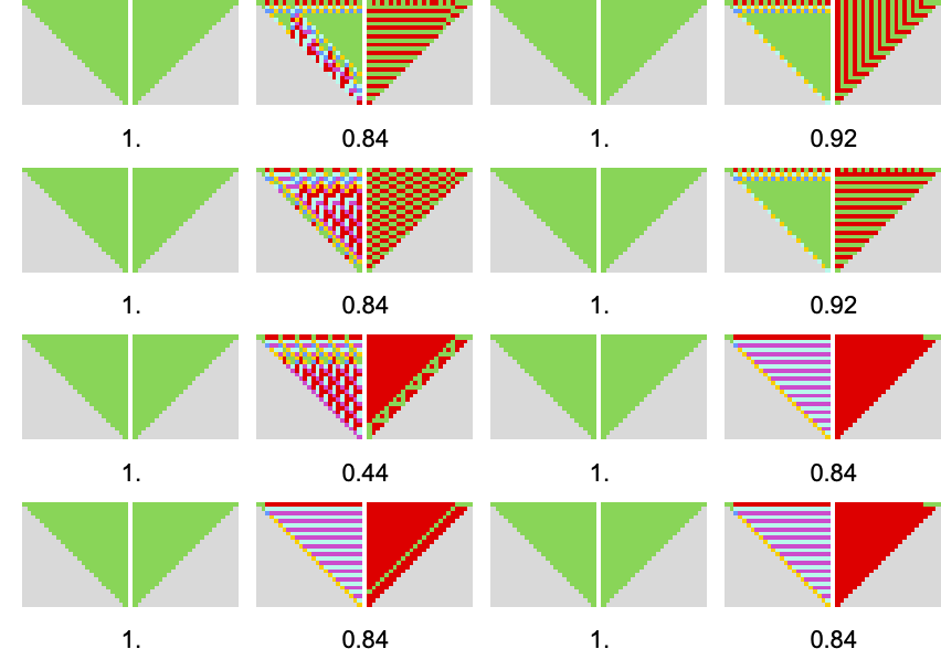
So what happens if pairs of these machines compete? Here are a few examples, where in each case we’re identifying the average payoff (here for 10 rounds of the match-or-not game):
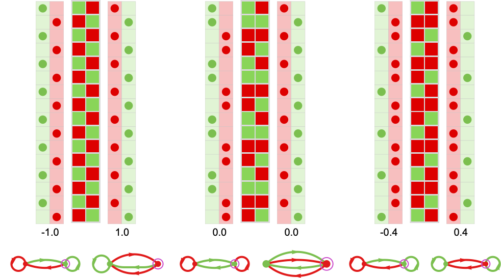
(In all competitions between pairs of finite state machines, the sequence of moves ultimately has to become periodic—with a period equal at most to the product of the number of states in each machine.)
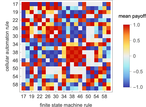
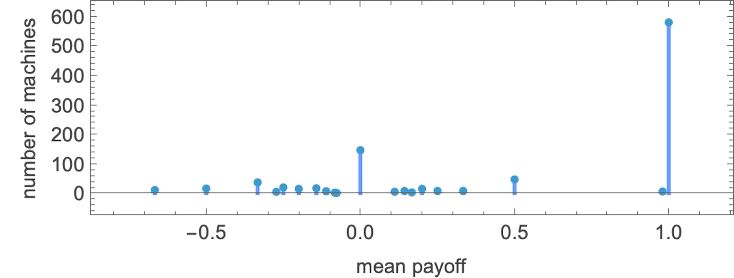
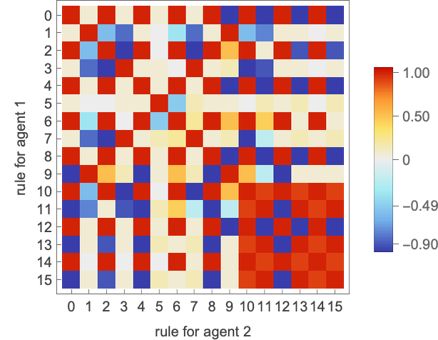
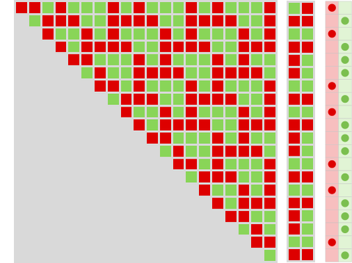
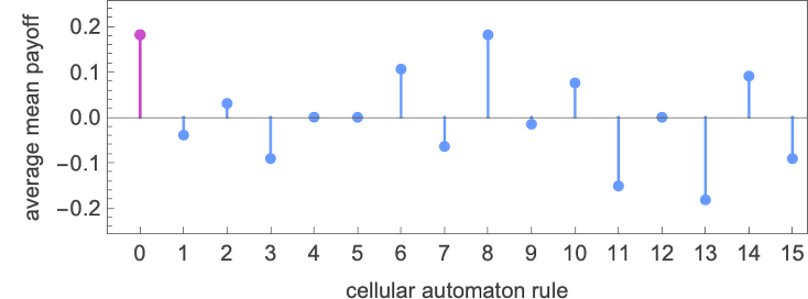
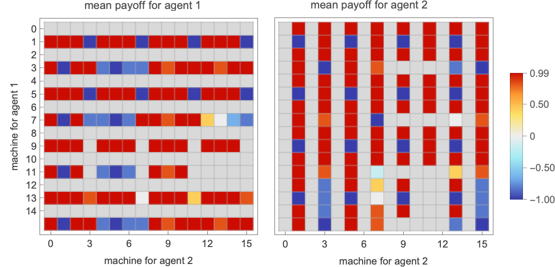
What happens if each of the 22 distinct 2-state machines competes against each of the other ones? We can summarize the results by showing the mean (long-term) payoff for every pair of machines (the payoff is for each machine “playing as agent 1”; in match-or-not, the payoff is negated if “playing as agent 2”):
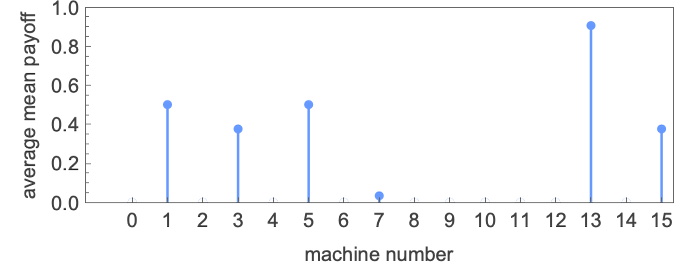
So what machine is the “overall winner”? One way to assess this is to look at the average of the mean payoffs achieved by a given machine when competing with all other (distinct) machines:
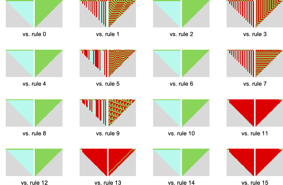
The winner by this measure is then machine 26:
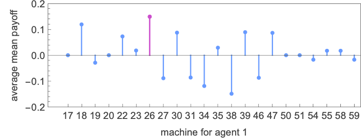
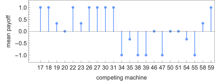
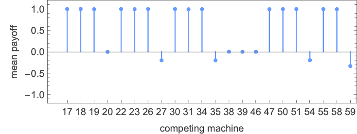
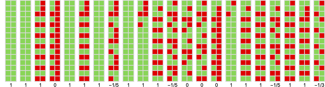
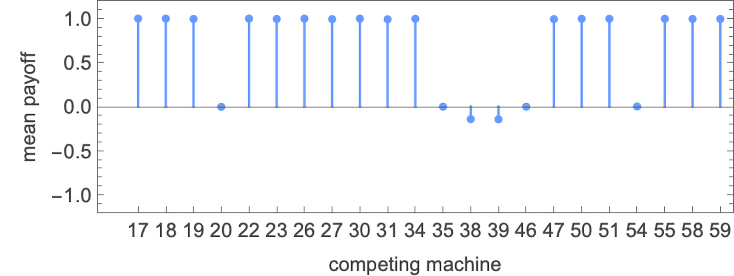
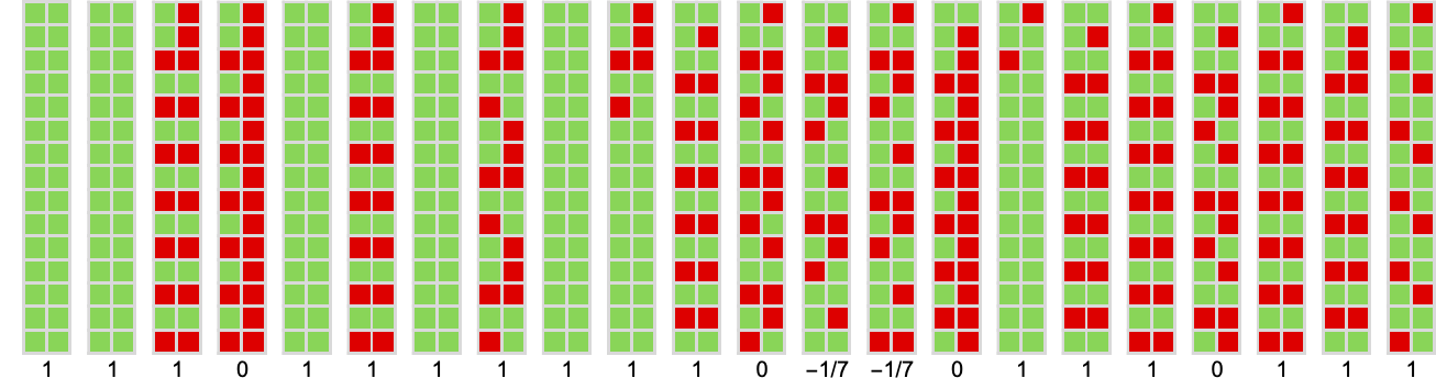
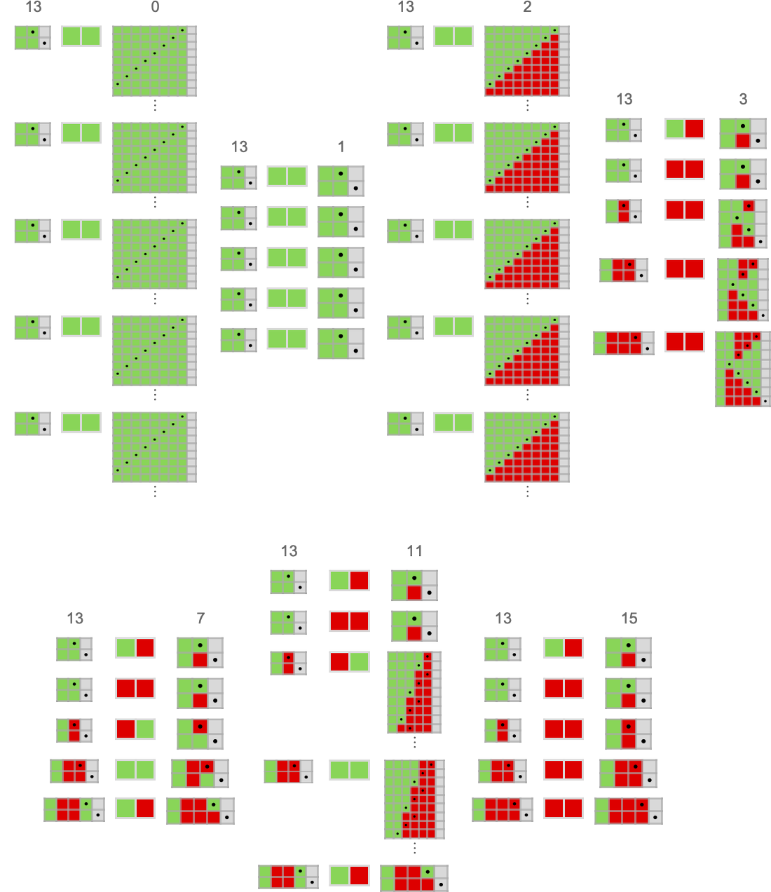
Running this machine against all (distinct) 2-state machines we get the following mean payoffs:
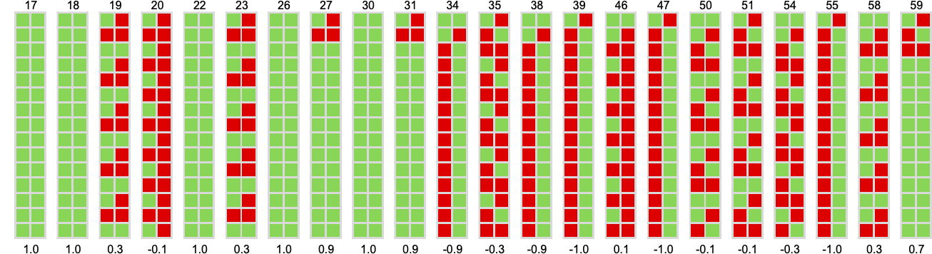
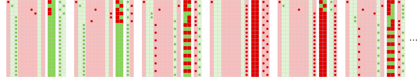
The actual behavior in each case—which doesn’t itself depend on the payoffs, only on the machines involved—is:
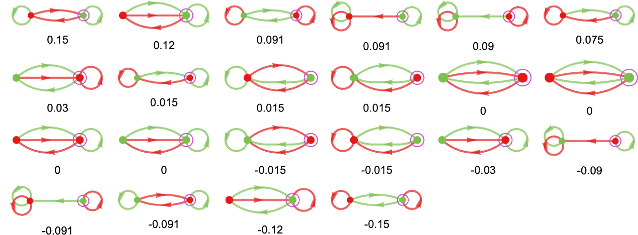
What are the “runners-up” to the winning machine? Here are all the distinct machines, ranked by their mean payoffs:
Here’s what happens if we play the top 3 runners-up against all machines:
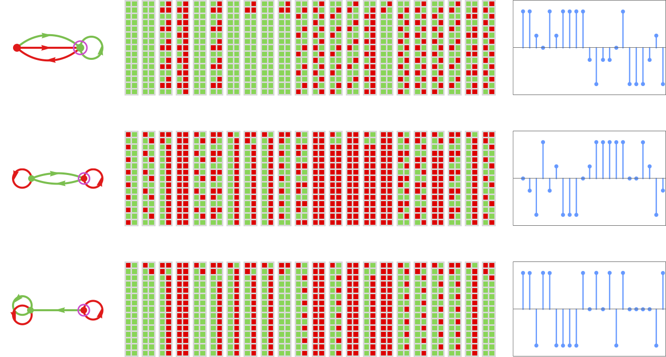
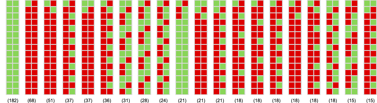
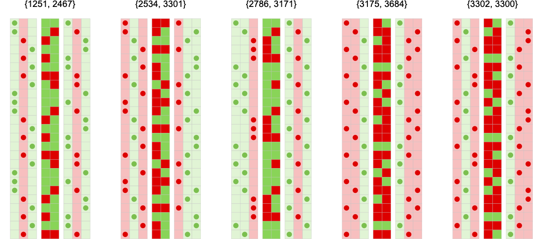
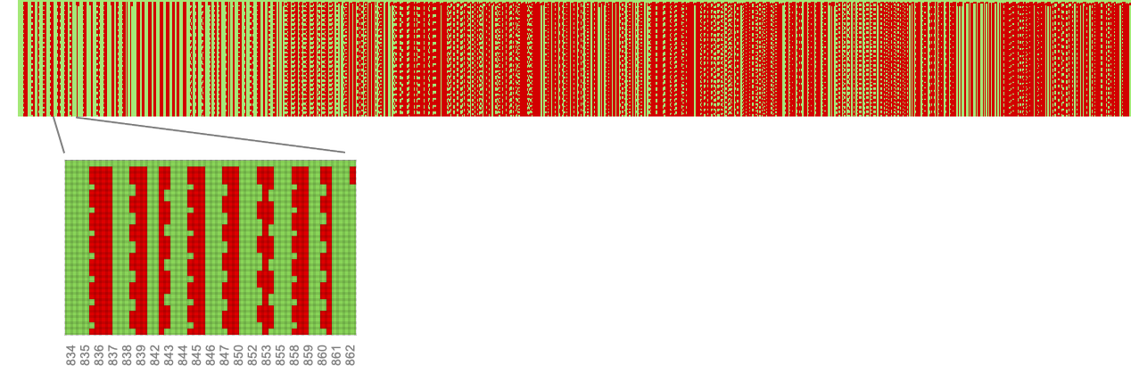
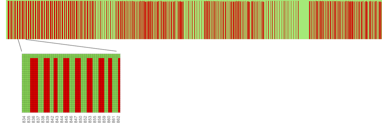
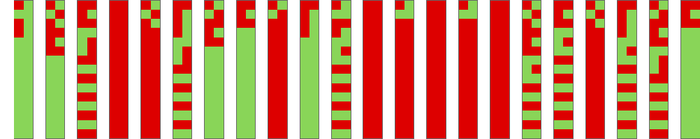
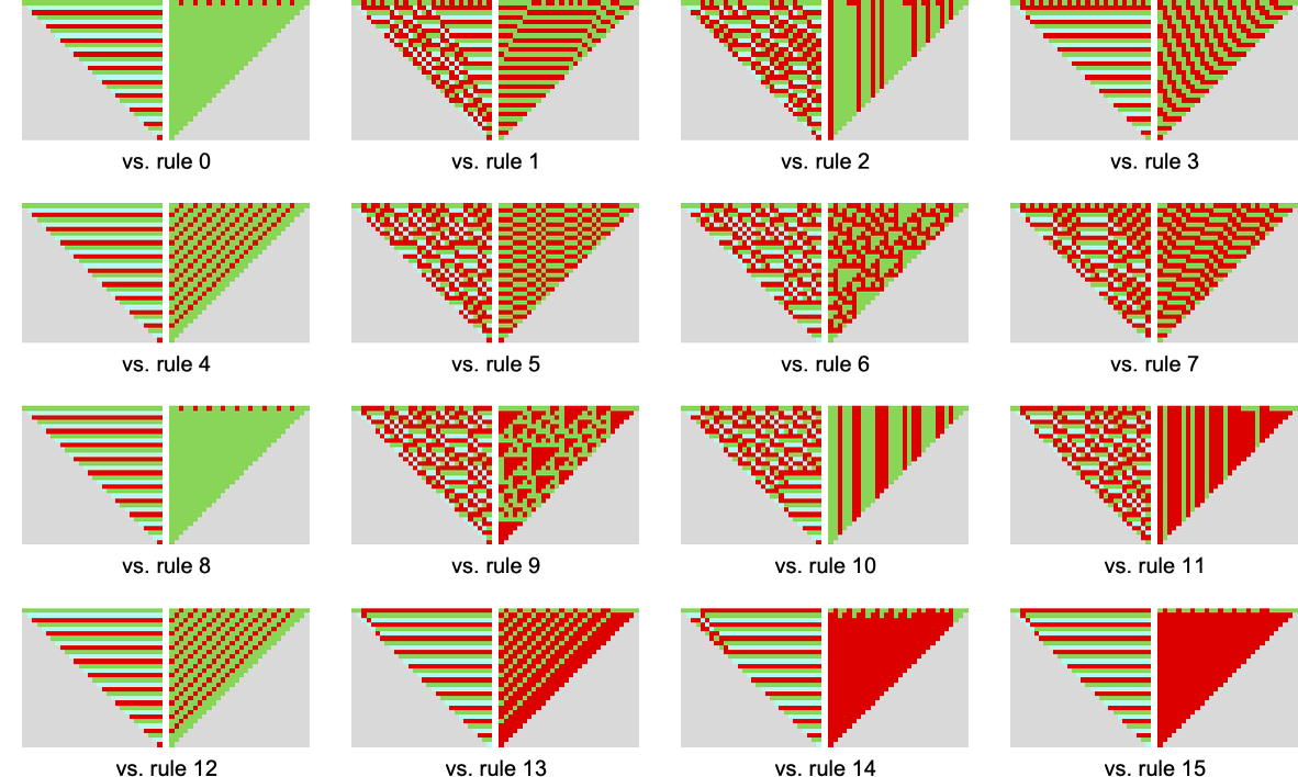
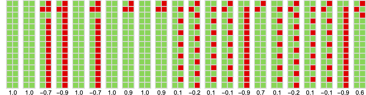
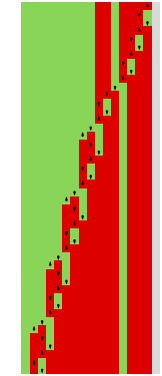
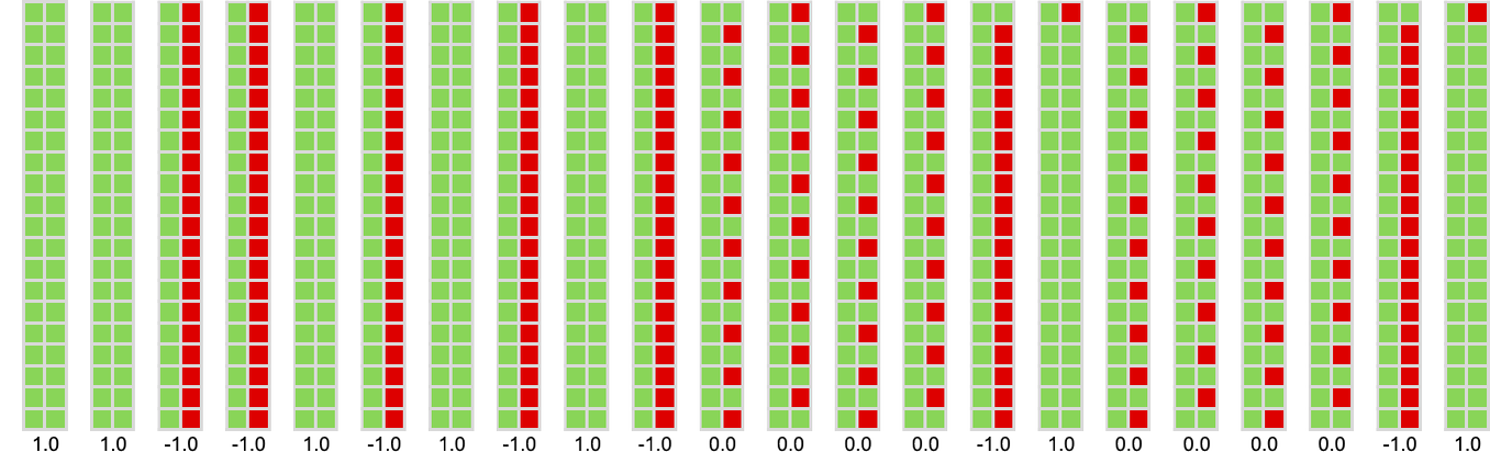
We can summarize how a machine behaves by showing the history of its behavior when playing against all other machines (or, in effect, by putting together the first columns in pictures like the ones above). Here are the results for all the machines (for 15 steps), ordered from highest average score down:
(Once again, these pictures are completely determined just from the machines involved; the payoffs in the match-or-not game determine only their ordering.)
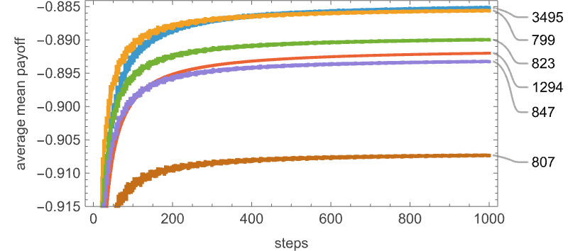
One footnote to what we’ve been saying here has to do with how many steps of competition we are getting the machines to do. For all finite-state machines, the behavior must eventually become periodic—and for 2-state machines the maximum period is 4 steps, with a maximum transient of 3 steps. But the actual average mean payoffs vary with the total number of steps one considers:
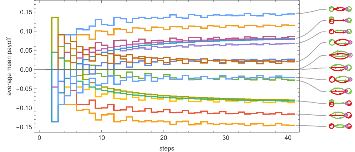
It’s notable that at the least for the first few steps, the rankings move around:
But in this case it doesn’t take too many steps for the ultimate winner to be clear (later on we’ll see examples where it takes much longer).
(There are other subtleties as well. One of them is that we are computing average payoffs by playing every machine against every other distinct machine. In principle we could also include other equivalent machines—which would slightly change the weighting of our averages. But since we’re really concerned with strategies, not machines as such, the scheme we’re using seems more appropriate.)
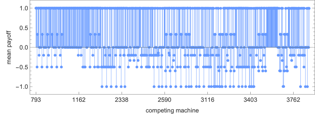
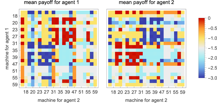
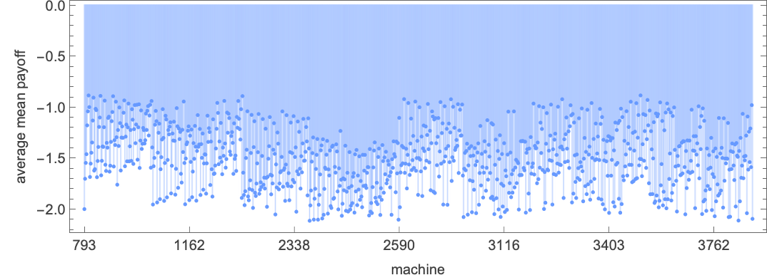
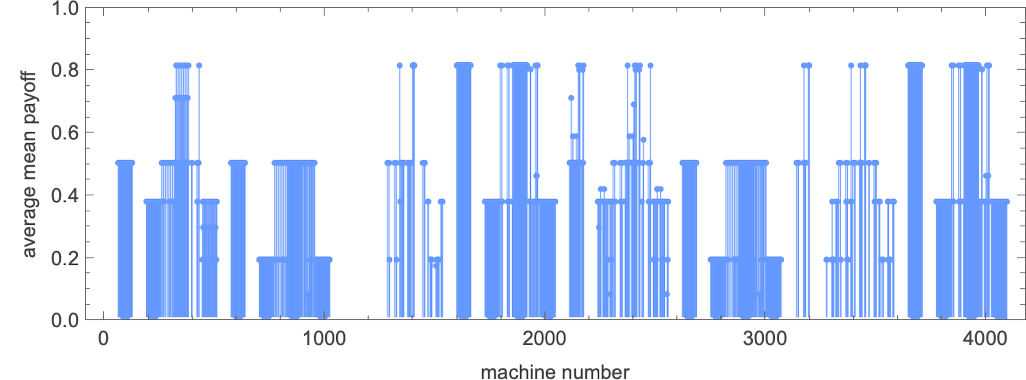
For the 956 distinct machines with s = 3 states, the corresponding “competitive array” (after 1000 steps) is:
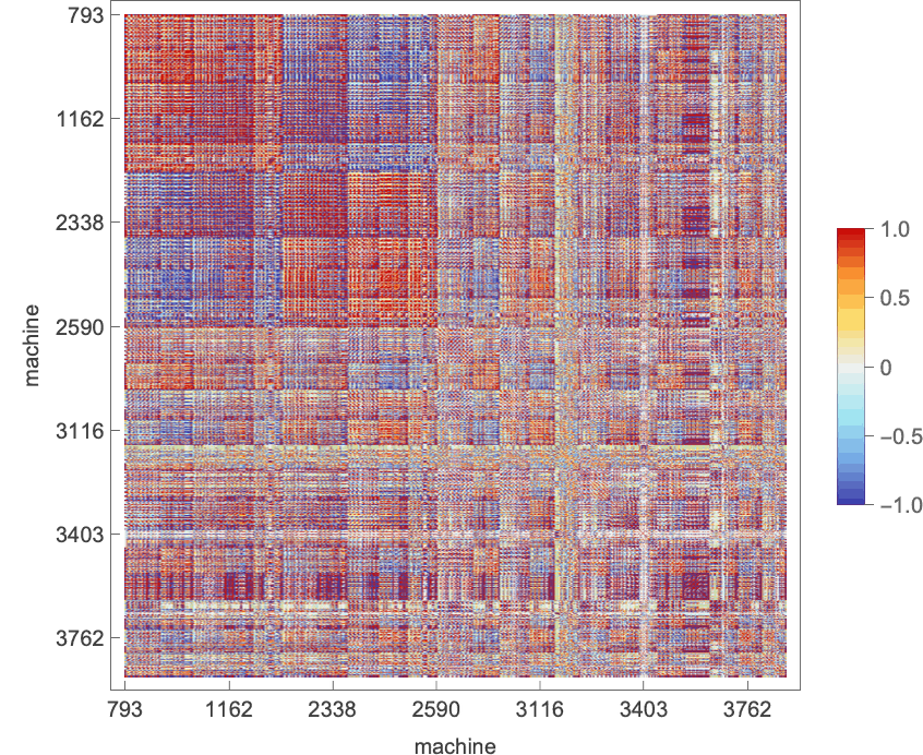
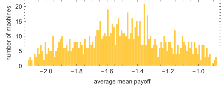
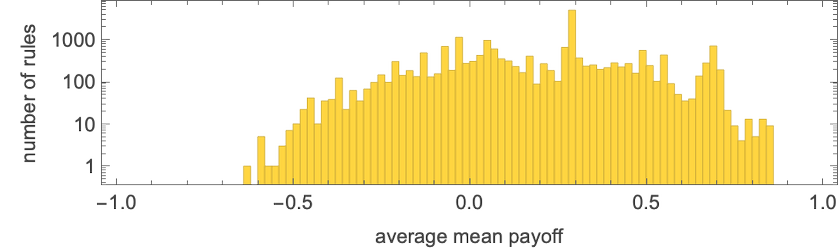
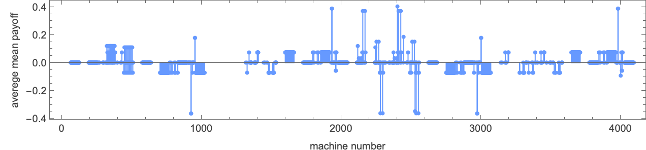
The average mean payoff for each of the machines (i.e. the average across each row in the “competitive array”) is then
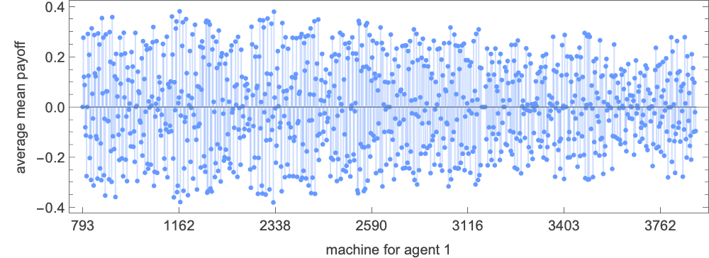
while the distribution of these average mean payoffs is:
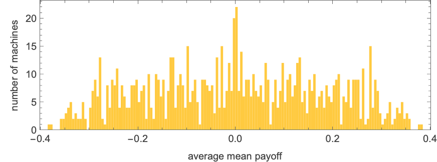
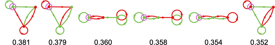
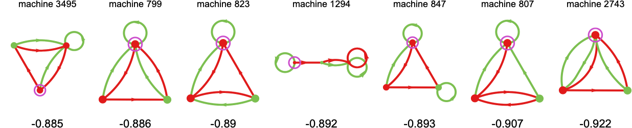
The top few machines for the match-or-not game are then:
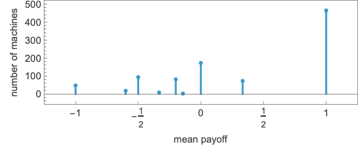
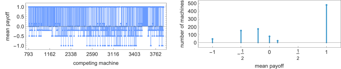
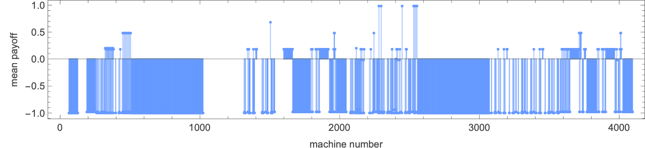
Running the top machine (s = 3 machine 1164) against all (distinct) 3-state machines we get the following mean payoffs:
The distribution of possible limiting mean payoffs here is:
And the most common forms of behavior seen are:
The maximum possible period for a competition between two 3-state machines is 9. Machine 1164 never quite achieves this; its maximum period of 7 occurs when competing with machines 2546 and 2755 (both giving limiting mean payoff –1):
If one looks at all possible pairs of 3-state machines, there turn out to be 792 that yield period-9 behavior, examples being:
(These have no transients; the maximum transient for 3-state machines turns out to be 8.)
We’ve talked about how a machine does “on average” when competing with all other (distinct) machines. But what do we mean by “on average”? So far, we’ve taken the “average” to be the mean of the payoffs obtained by competing with each other machine (and the payoffs here are themselves means across successive steps). But what if we use the median instead of the mean? Here are the median payoffs from running each machine for 1000 steps against all other machines:
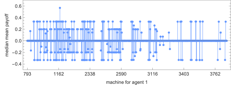
The standout winning machine here is machine 1172:
The mean payoffs and their distributions in this case are:
And the median is “anomalously high” because with this machine exactly 1/2 of all mean payoffs are +1. (The corresponding mean is pulled down by the “left tail” in the distribution of mean payoffs.)
Let’s look (basically as above) at the actual behavior of each of the distinct 2-state finite state machines when competing against all other 2-state machines, ordered from smallest average mean payoff to largest:
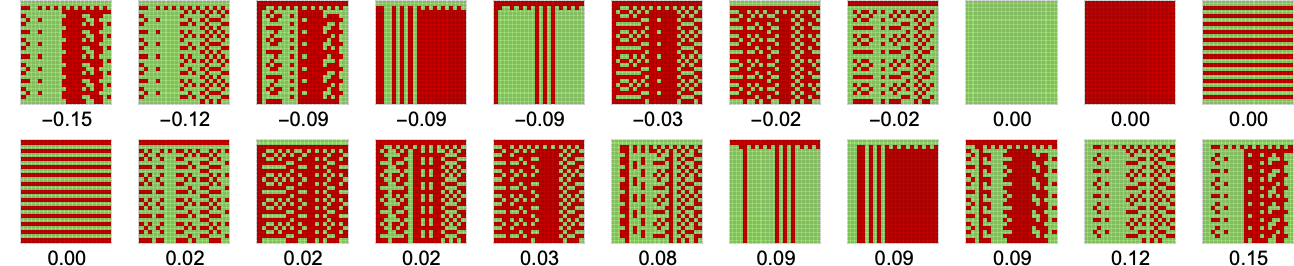
The cases with 0 average mean payoff look simple in their behavior. But for other average mean payoffs, the behavior of a given machine competing against all others seems more complicated.
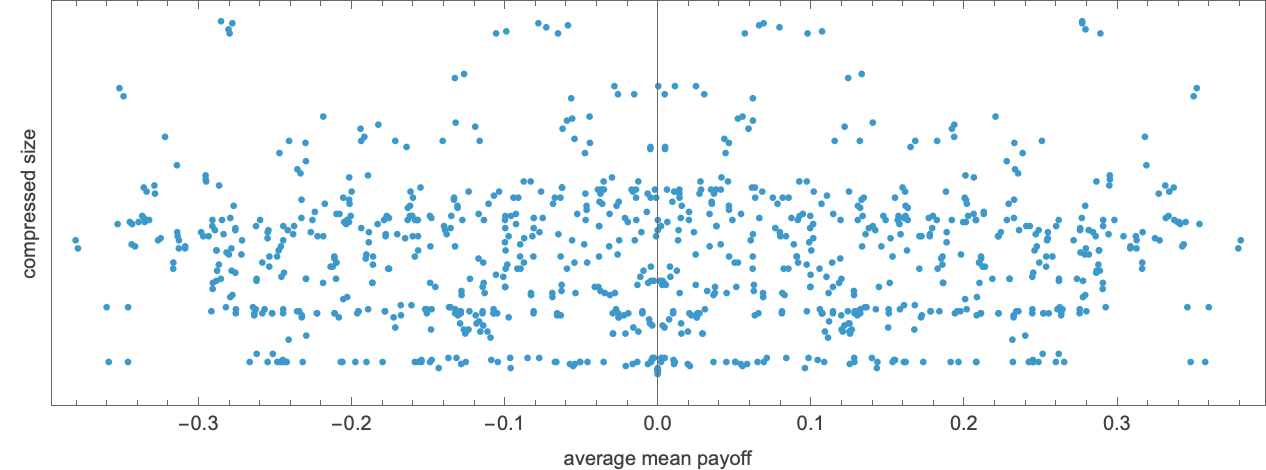
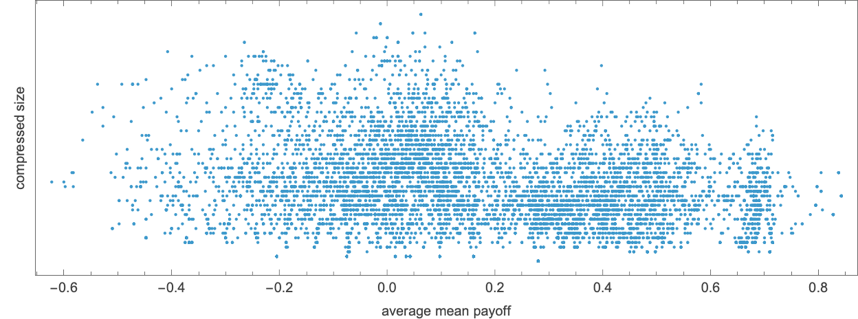
We can get some sense of this complexity by looking at the compressed size (as obtained from Compress) of the array of behavior shown above:
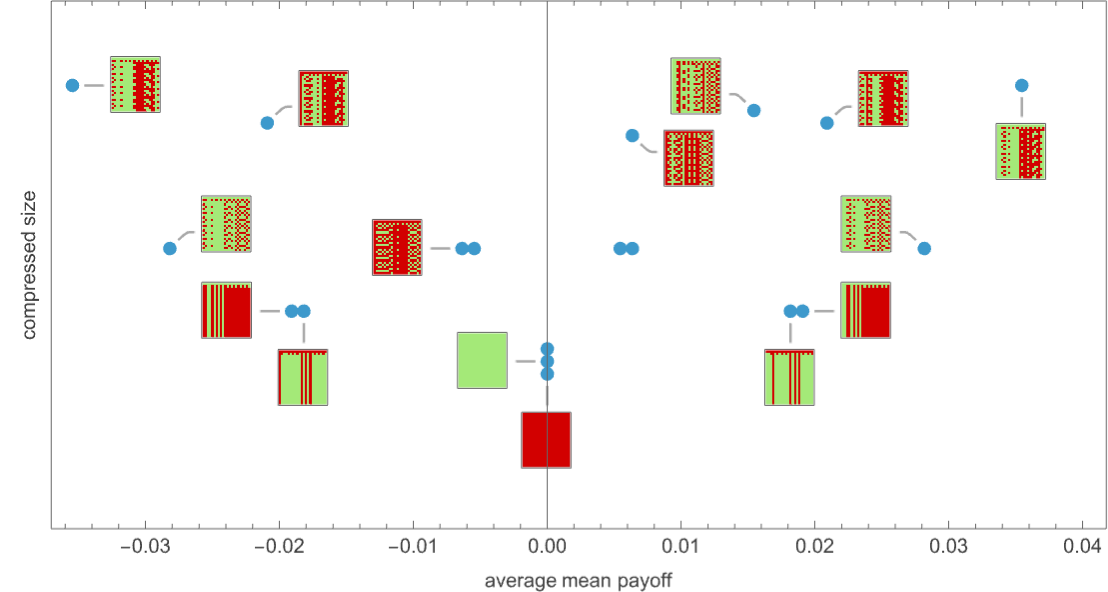
Here’s the corresponding result for the 956 distinct 3-state machines—showing no strong correlation between average mean payoff and our estimate of the complexity of behavior:
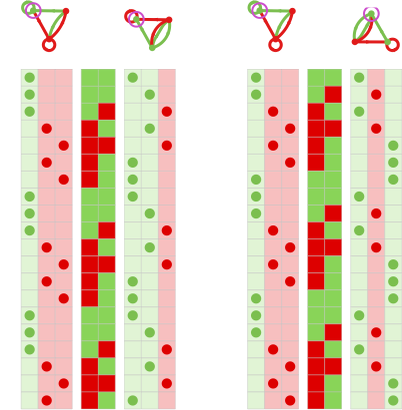
And indeed among machines with the highest average mean payoffs there is still quite a diversity of levels of complexity in behavior
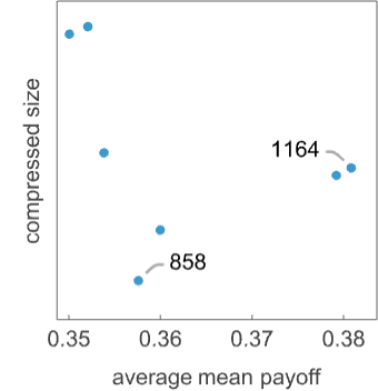
with the “behavior traces” of the machines indicated being
and
In other words, at least in this case, we really can’t say that winning machines are characterized either by being particularly complex in their behavior, or particularly simple. It seems that it’s detailed structure, rather than overall features, that determines what machines will win.
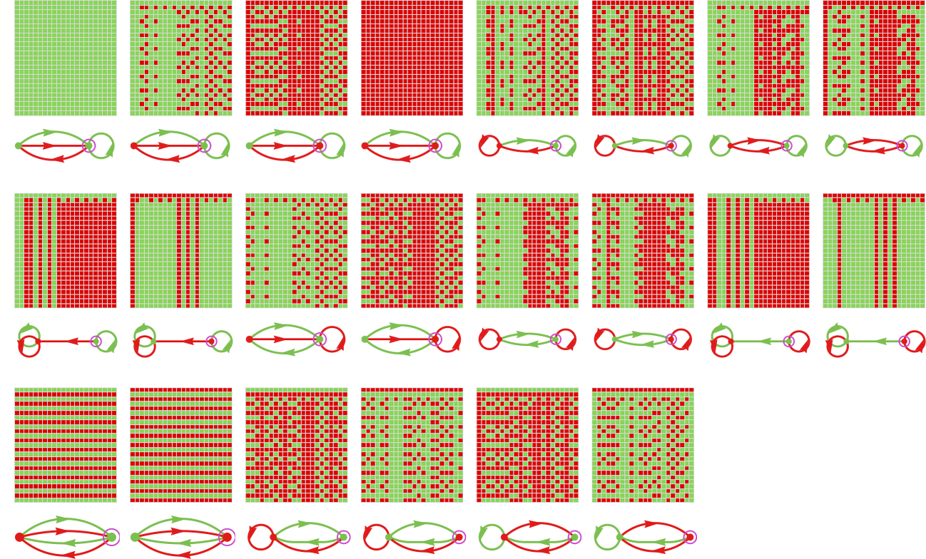
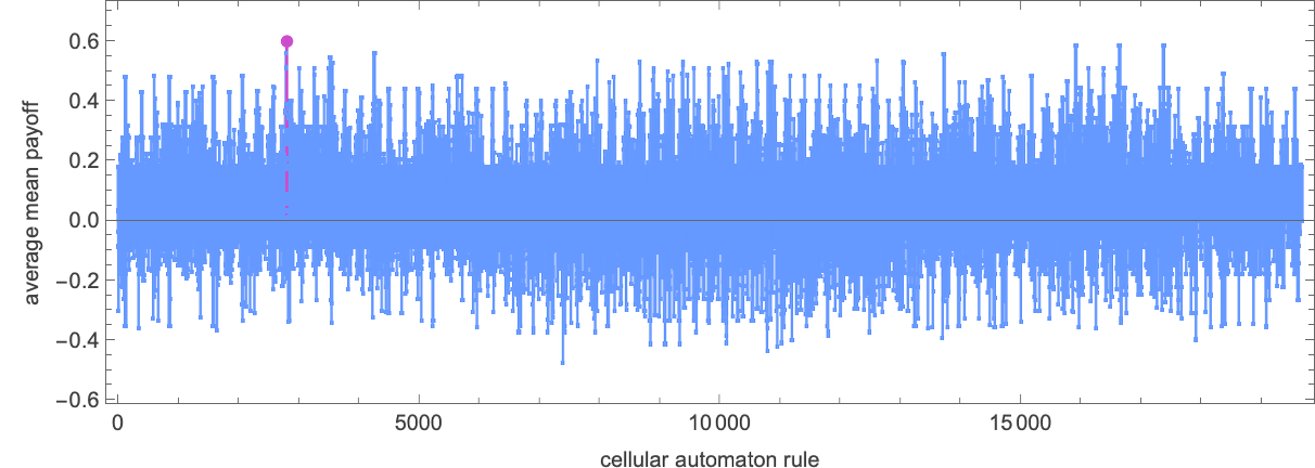
Can finite state machines with more states systematically do better (i.e. achieve larger payoffs) than ones with fewer states? The best average mean payoff any 2-state machine can achieve when competing with all other 2-state machines is about 0.151. But if, for example, we consider 3-state machines competing (for 1000 rounds) against 2-state machines, the best average mean payoff is instead 0.593:
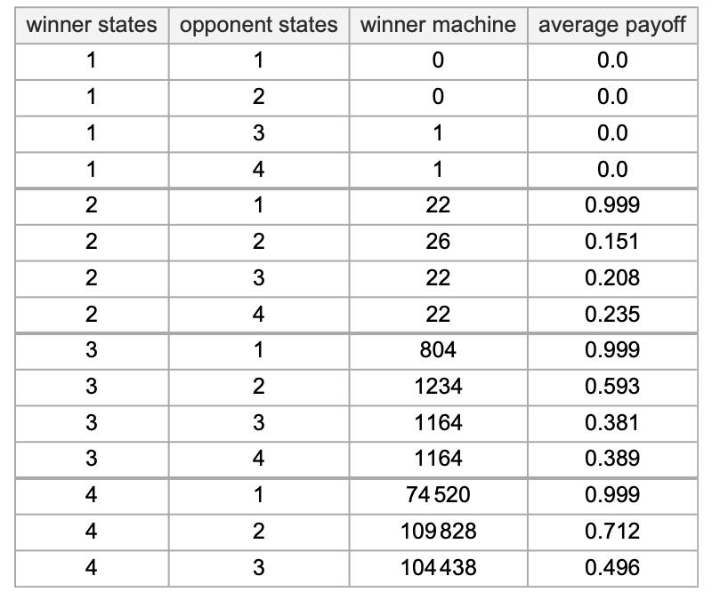
Looking at the distribution of possible average mean payoffs, we see that the distribution of average mean payoffs is wider for 3-state machines than for 2-state ones—a fact that is at least partly just a consequence of there being many more possible 3-state machines than 2-state ones:
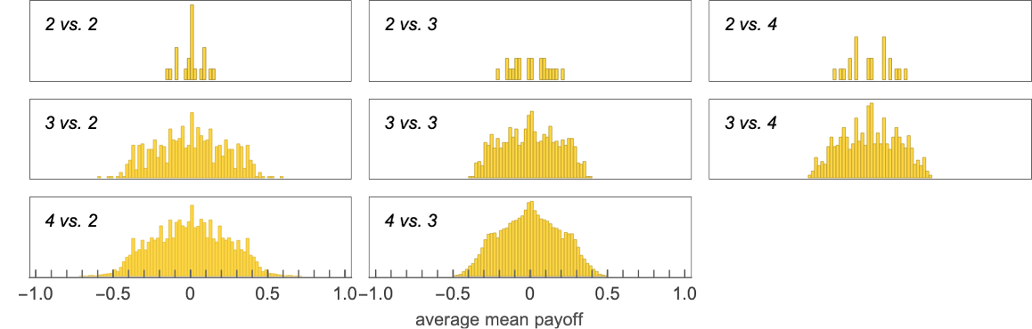
But something that’s notable is that the very broadest distribution is for 3-state machines competing against 2-state ones: in effect it seems that with their larger collection of possible strategies, the 3-state machines can do better at “outmaneuvering” the 2-state ones.
The 3-state machine that does the best overall against 2-state machines is machine 1234:
It doesn’t always definitively win (with mean payoff +1), but does so the majority of the time:
How does it achieve this? Basically, for lots of different 2-state machines, this particular 3-state machine manages to behave just as they do:
In some sense, there are facets of the 3-state machine that “resonate” with many 2-state ones:
How about 4-state machines? The 4-state machine that does best overall against 2-state machines is machine 109828:
Out of the 22 2-state machines, it only gets less than payoff +1 in 6 cases:
Here’s the behavior for all 22 cases:
And once again we can think of the 4-state machine as successfully “covering” most of the 2-state behaviors:
In many practical situations where there’s competition, there’s a way for the agents that are competing to evolve. So can we make a minimal model of this using finite state machines?
In what we’ve done so far, we’ve always been looking at a space of all possible finite state machines. But what about sequences of machines found by adaptive evolution? Is there, for example, a way to adaptively evolve machines to do progressively better in competitions?
The first step in doing this is to see how we might make successive mutations to finite state machines. A simple approach is to say that any given mutation can affect either a random vertex or a random edge in the graph of a machine. For a vertex, the mutation just reverses its color. For an edge, it either reverses the color, or “reroutes” the edge to a different vertex (with the constraint that doing so doesn’t disconnect the graph). Applying a sequence of such mutations at random gives for example
or, with a different graph rendering:
(Note that we’re mutating machines in whatever form we find them; we’re not worrying about equivalences between machines, or the canonicalization of machines.)
Imagine we have an opponent machine—like 3-state machine 1165—that usually forces a lose, i.e. limiting payoff –1 (for example about half the time when competing with other 3-state machines):
Now we can ask whether we can adaptively evolve a machine that will win against this opponent. In order to give our adaptive evolution process some “room to maneuver” we’ll use a 4-state machine. We can start with a random such machine, say
which “loses” (always having payoff –1) against machine 1165:
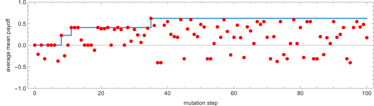
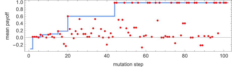
To do adaptive evolution, we now make successive random mutations to this machine, “accepting” a mutation if it doesn’t decrease the mean payoff, and otherwise rejecting it. The result is a typical “fitness curve” in which most mutations (indicated by red dots) don’t lead to improvement in the payoff—but there are some that lead to “breakthroughs” where the payoff increases (sometimes only by a small amount), with the payoff eventually reaching the maximum value of +1:
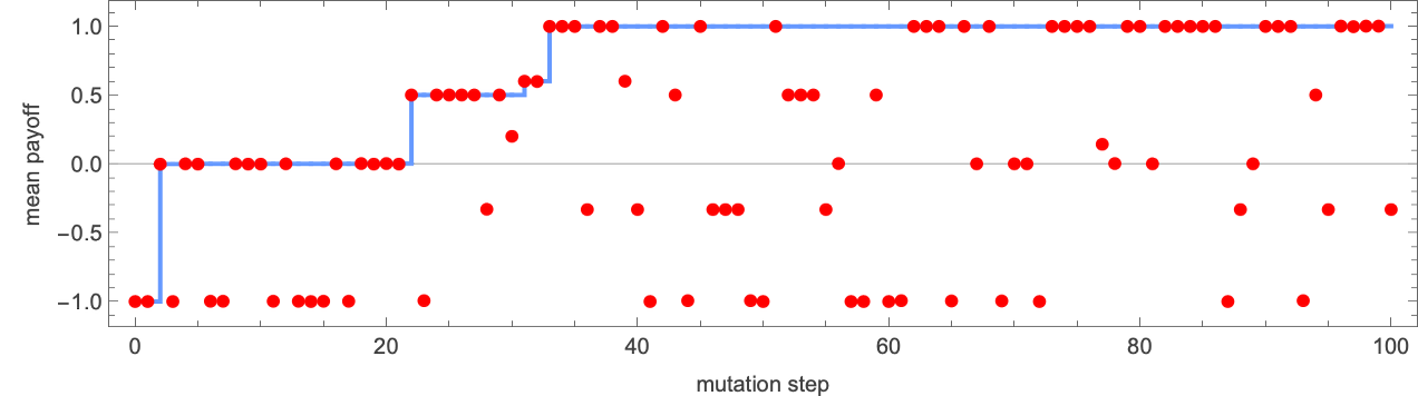
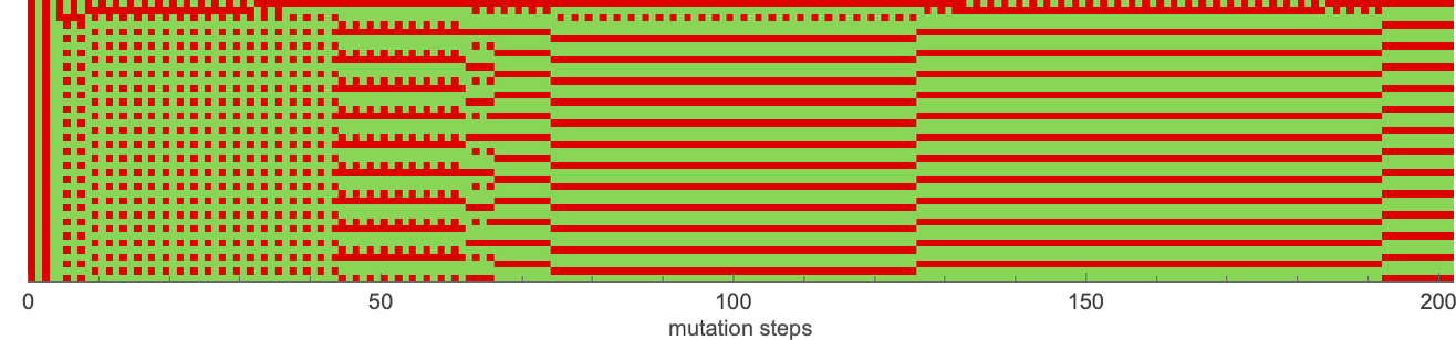
The various “breakthroughs” progressively converge on a “perfect solution” with payoff +1:
Concatenating the successive results over the course of the adaptive evolution process, we can see the eventual convergence to the perfect solution where the actions of the two agents always match:
With different random mutations, the “fitness curve” will be different in detail, though will have the same general form. And the same is true with different specific opponents.
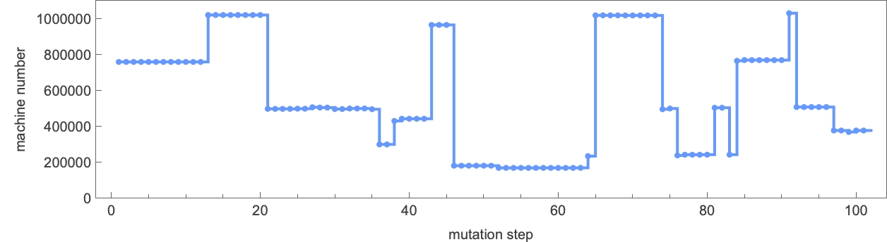
By the way, using our way of numbering finite state machines, we can make a plot of how the process of adaptive evolution “moves the machine around in rule space”:
But what happens if we do as we have done above, and ask about the mean payoff averaged over all possible finite-state-machine opponents of a given size? For example, how well can 4-state machines do against all possible 2-state machines?
Starting with the same random 4-state machine as before, a typical fitness curve is:
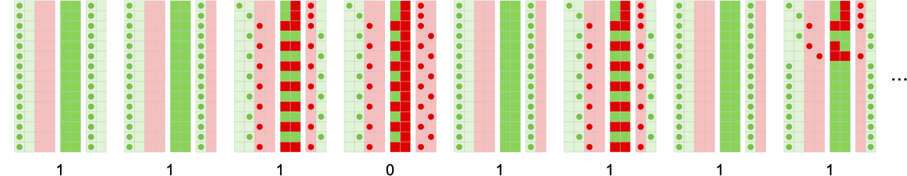
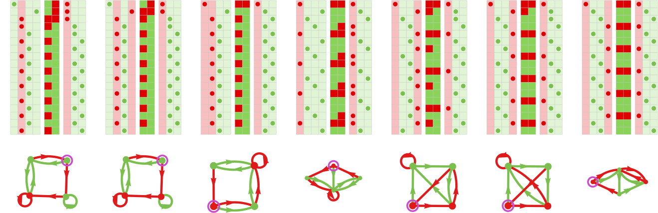
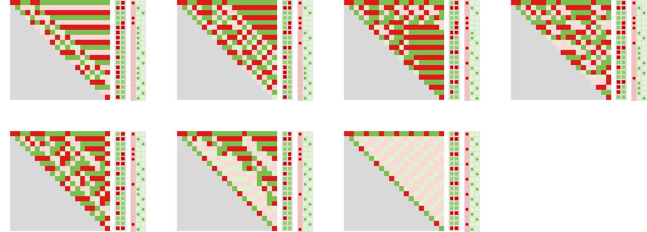
The fitness here increases, but never reaches +1. The behavior of successive “breakthrough” machines playing against all size-2 machines is:
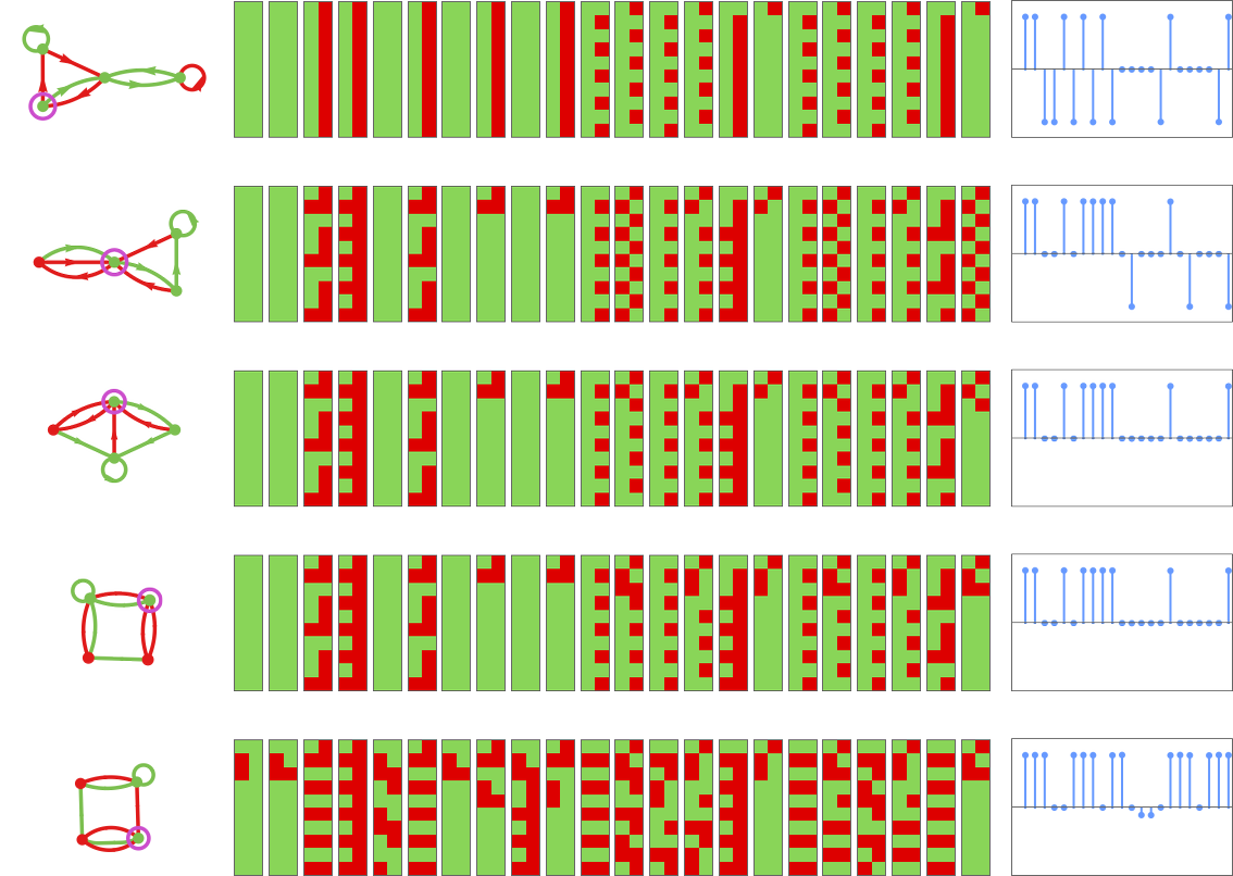
And we can see that even the best machine we get still loses to some of the 2-state machines, yielding in the end an average mean payoff of about 0.62.
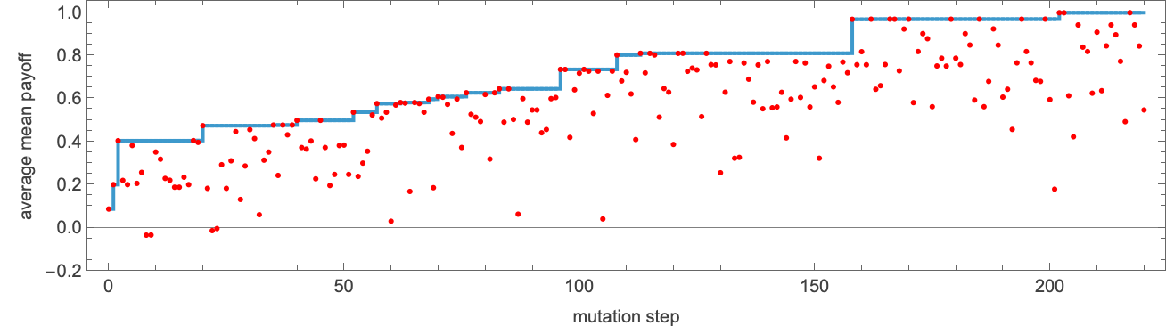
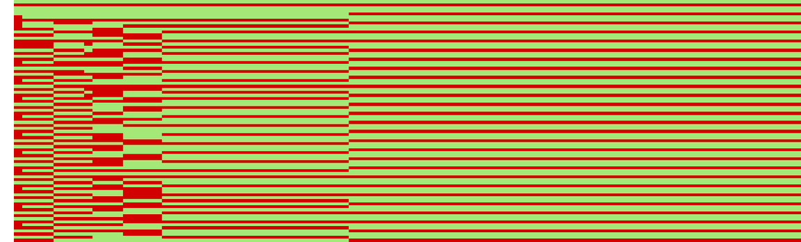
So what happens if we look at machines that have more states? With 10 states, for example, it is possible to adaptively evolve to a machine that achieves limiting payoff +1 against every single 2-state machine:
The final machine obtained in this case
can be thought of as a kind of (2-state) “universal winner”—that ultimately wins against all 2-state machines:
How does it do it? In some sense the machine is big enough that it can have different “specialized parts” for different opponents. And if we look at how the machine behaves we indeed see that with different opponents the machine settles into different subsets of its complete space of states:
And even if we consider all 956 3-state machines as opponents, our machine continues to do well. It doesn’t win in all cases, but it still achieves an average mean payoff of +0.603:
Some examples where the machine doesn’t win—in effect because it doesn’t contain as a submachine something to deal with a particular opponent—include:
So far we’ve considered the adaptive evolution of a single machine competing either against a single fixed opponent, or against a collection of fixed opponents. But what if both the machine and its opponent are undergoing adaptive evolution?
For example, let’s say that on alternating adaptive evolution steps we do a mutation on a machine and on its opponent. We keep the mutation for each machine if the (mean) payoff for that machine does not decrease; otherwise we reject it.
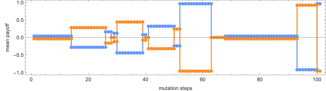
With this setup, here’s the evolution of mean payoffs for two (initially identical) 4-state machines:
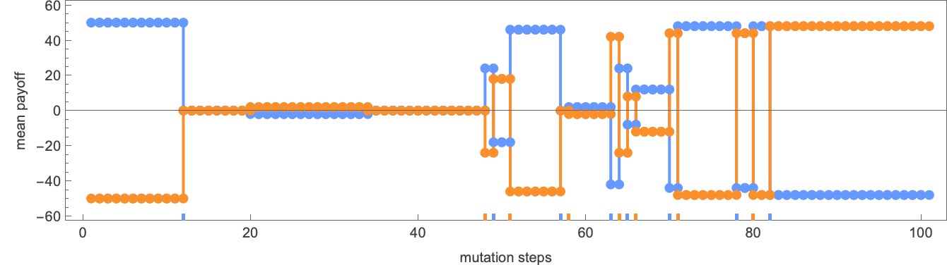
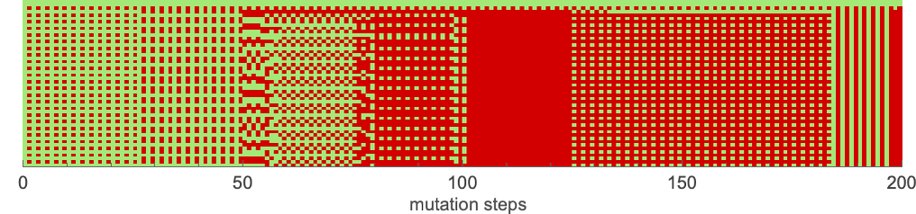
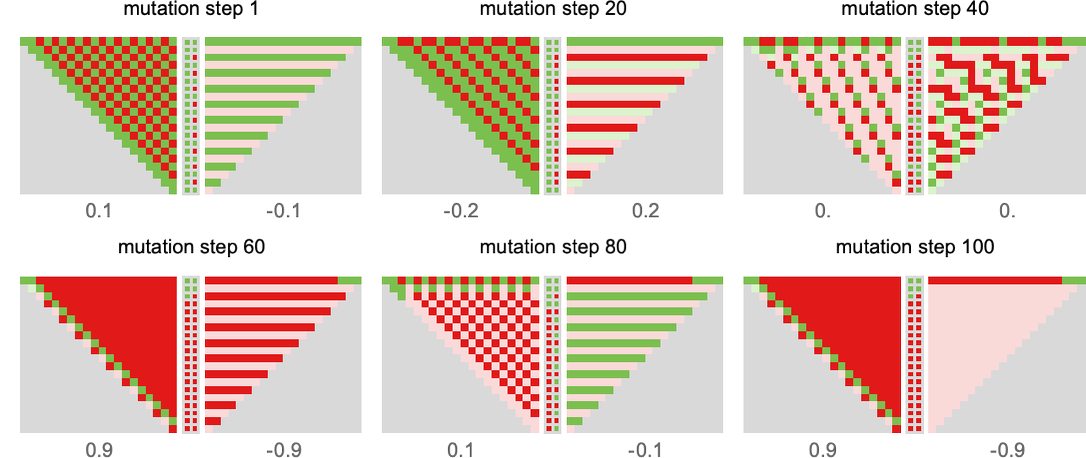
There are periods where one machine wins, and periods where its opponent wins—as visible in the actual successive behaviors of the machines:
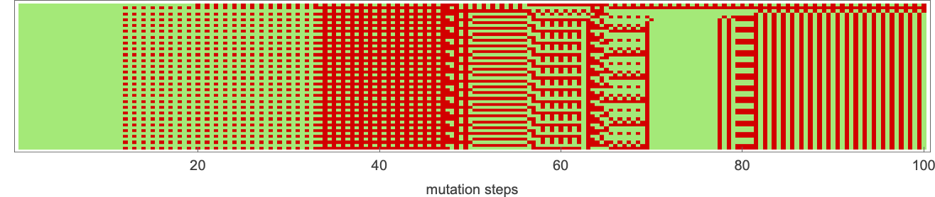
The actual machines found by adaptive evolution move around in rule space—soon losing memory of what they initially were:
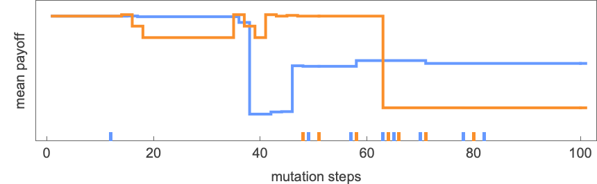
Not much changes if the number of states in the machines change, or aren’t the same—though there is typically less alternation of winners for machines with more states, presumably because each individual mutation tends to have less effect on behavior if there are more states.
Everything we’ve done so far has been based on the particularly simple game of match-or-not (“matching pennies”). So what happens with other games? And in particular with the famous “prisoner’s dilemma” game? Here are the payoffs for this game
where in the usual narrative for the game one interprets ![]() as “defect” and
as “defect” and ![]() as “cooperate”.
as “cooperate”.
Just as above, we can imagine defining strategies for the prisoner’s dilemma game based on finite state machines. Here are a few examples of iterated games between 2-state machines—now with payoffs determined by the prisoner’s dilemma game:
In the case of match-or-not, it was visually easy to tell whether a particular payoff was ±1 or 0 just by seeing whether the actions of the agents matched at a particular step. Here it’s not quite so visually obvious.
But using the payoffs for the prisoner’s dilemma game we can compute the cumulative payoffs for these examples (and, unlike in match-or-not, which is a zero-sum game, the payoffs for the two agents don’t sum to zero at each step):
Much as we did before, we can now consider competitions between agents whose strategies are based on all possible 2-state finite state machines (for match-or-not the zero-sum nature of the game makes the resulting array of payoffs symmetrical; here there’s symmetry only from the fact that the payoffs remain the same if one interchanges the roles of agent 1 and agent 2):
With this setup, we can now ask what machine is the “overall winner”—say in the sense that it has the largest average mean payoff playing against all other (distinct) 2-state machines:
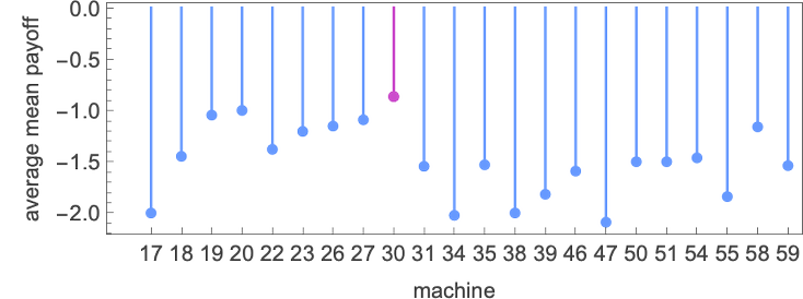
The answer turns out to be machine 30:
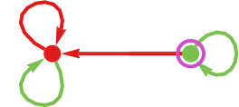
In the literature of prisoner’s dilemma this is often called “grim trigger”, because it yields a strategy that starts with ![]() , then repeats this until its opponent first gives
, then repeats this until its opponent first gives ![]() —after which it always gives
—after which it always gives ![]() .
.
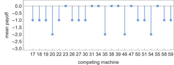
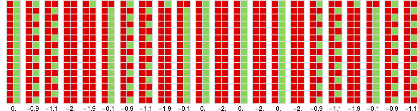
Running this machine against all other 2-state machines we get the following behaviors
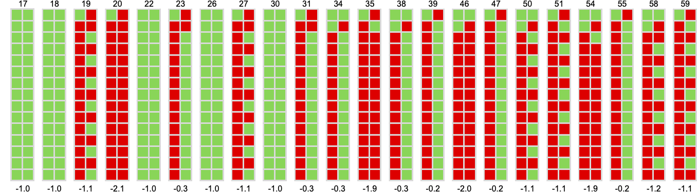
corresponding to the following mean payoffs:
Looking at the average mean payoff for all 2-state machines, the ranking of these machines is:
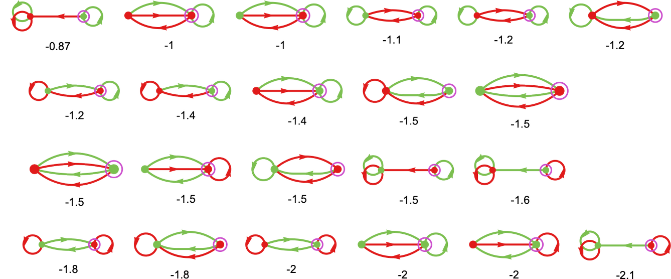
It’s notable that machine 22 (which corresponds to the famous “tit-for-tat” strategy)
is quite far down in this ranking, even though it’s often identified as the most successful in collections of human-suggested strategies.
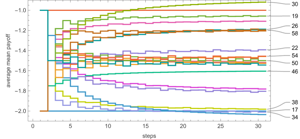
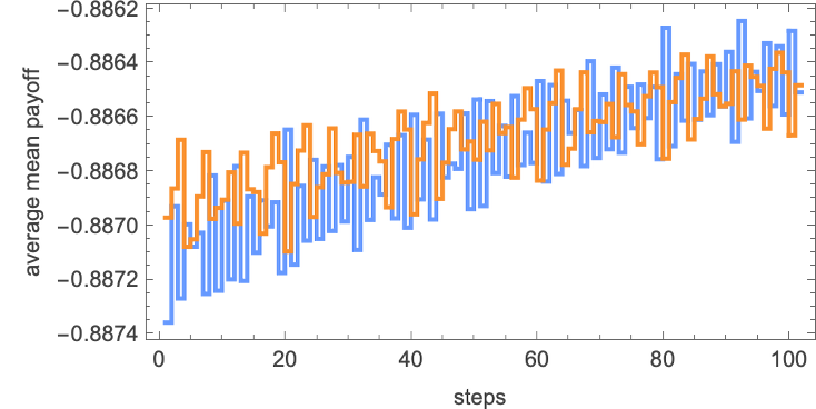
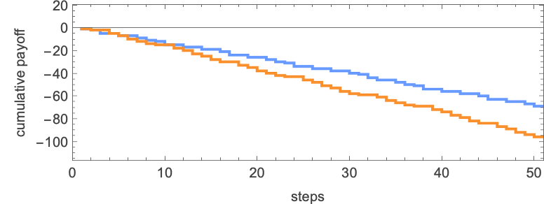
The rankings we’ve just given are based on average mean payoffs obtained after many iterations of the prisoner’s dilemma game. But if we do only a few iterations, the rankings can be different:
Zooming in at the beginning we can then see that machine 30 only starts to win after 13 steps:
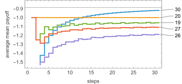
Machine 20 gives a constant average mean payoff of –1 obtained from
while machine 30 yields an average mean payoff given by –![]() –
– ![]() , limiting to –
, limiting to –![]() ≈ –0.86.
≈ –0.86.
So what about 3-state machines? This gives the average mean prisoner’s dilemma payoff for each of these machines:
The distribution of these average mean payoffs is:
The machines with the highest ultimate average mean payoffs are:
But this ordering emerges only after more than 500 steps
with the crossover of average mean payoffs being surprisingly complex:
(The seemingly quite random variation of average mean payoffs reflects the combining of many different periods in the always-ultimately-periodic behavior of competitions between machines.)
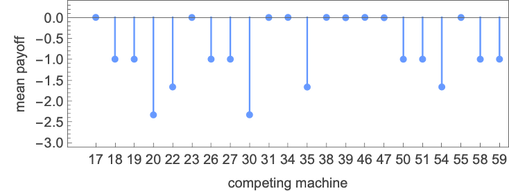
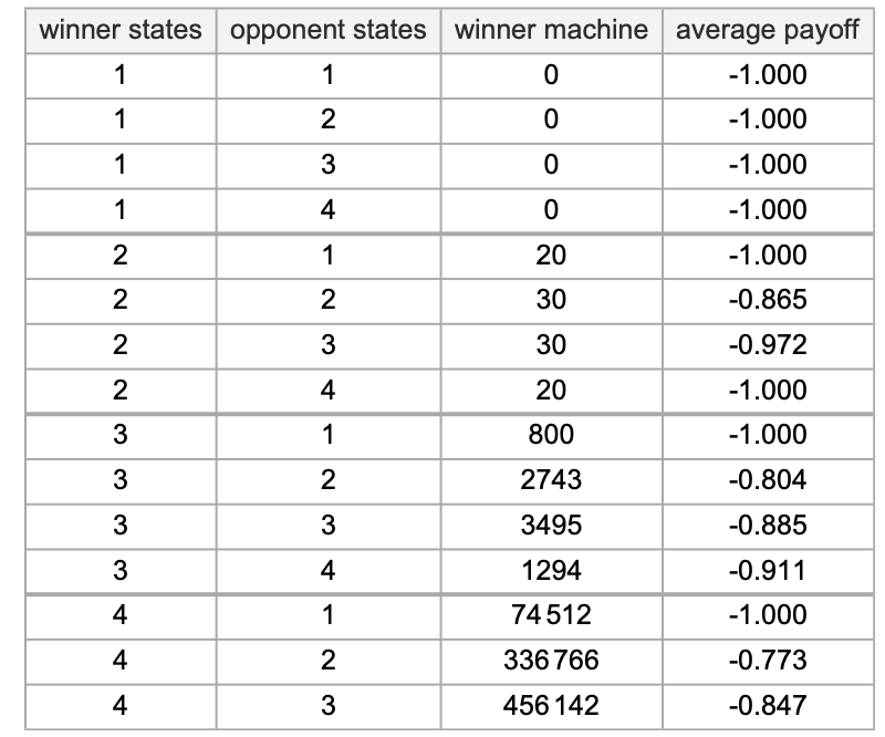
So how do 3-state machines do compared to 2-state machines in the prisoner’s dilemma game? Running 2-state machines against each other, machine 30 gets the highest average mean payoff of about –0.866. Meanwhile, for 3-state machines running against each other, the highest average mean payoff achieved is the very slightly smaller –0.885. What about 2-state machines running against 3-state ones? They don’t do well. Machine 30 does the best—but now it gives an average mean payoff not of –0.866 but instead of about –0.97.
But now, running 3-state machines against 2-state ones, the best average mean payoff is larger—about –0.80, as achieved by machine 2743
with the mean payoffs obtained by running it against each possible 2-state machines being:
How about 4-state machines? Running all these against 2-state machines, the overall winner is machine 336766 with average mean payoff –0.77:
The mean payoffs against each 2-state machine in this case

are very similar to those for the winning 3-state machine, the only different behaviors occurring when the opponents are 2-state machines 20 and 30:
Summarizing these results, the winning machines with small numbers of states that we’ve found for prisoner’s dilemma are:
But what about machines with more states—that we might find by adaptive evolution? Here’s an example of adaptive evolution for 10 states, competing against all 2-state machines:
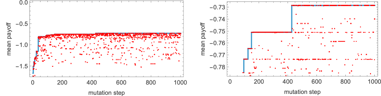
After 1000 steps of this adaptive evolution, we get the 10-state machine
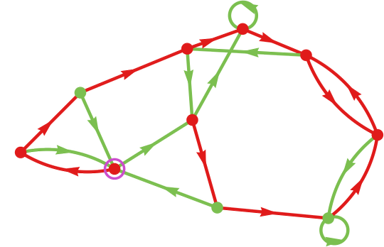
with average mean payoff –0.73.
The behavior of this machine competing with all 2-state machines is:
We’ve now looked at two specific examples of games—match-or-not and prisoner’s dilemma—and we’ve seen very similar phenomena in both cases. But what about other games?
If we allow payoffs –1 and +1 (as in match-or-not) there are a total of 256 possible games:
Of these, 16 are zero sum (like match-or-not)—in the sense that the sum of the payoffs for the two agents is always zero), and 16 are symmetric (like prisoner’s dilemma)—in the sense that the payoff for the two agents is always the same.
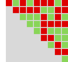
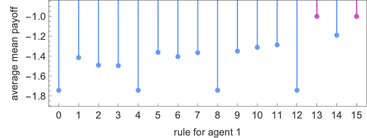
For each of the 256 possible games, we can compute the average mean payoffs for each possible 2-state finite state machine competing with all 2-state machines:
The winning average mean payoffs for these 256 games are always –1, 0 or +1:
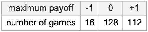
In most cases, many machines achieve the maximum payoff; across all games, this is the number of times each machine is a winner:
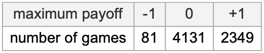
What about when we look at more games—for example ones with payoffs –1, 0, +1? There are 6561 such games. And the story is very much the same, with some slight differences:
Everything we’ve done here so far has been based on using finite state machines as our source of strategies. Now we’re going to turn to another source of strategies: cellular automata.
The setup we’re going to use takes the actions of our agents to be determined by running cellular automaton rules. The basic idea is that at each step the initial conditions for the cellular automaton are given by the sequence of actions taken by the opponent so far. The next action of our agent is then determined by the value of the cell obtained by running the cellular automaton for as many steps as there were actions taken so far by the opponent.
More specifically, let’s say the rules for our cellular automaton are:
And let’s say the actions taken by the opponent so far have been:
Then the idea is to run the cellular automaton with these as initial conditions
and to extract the final cell value to determine the next action to take.
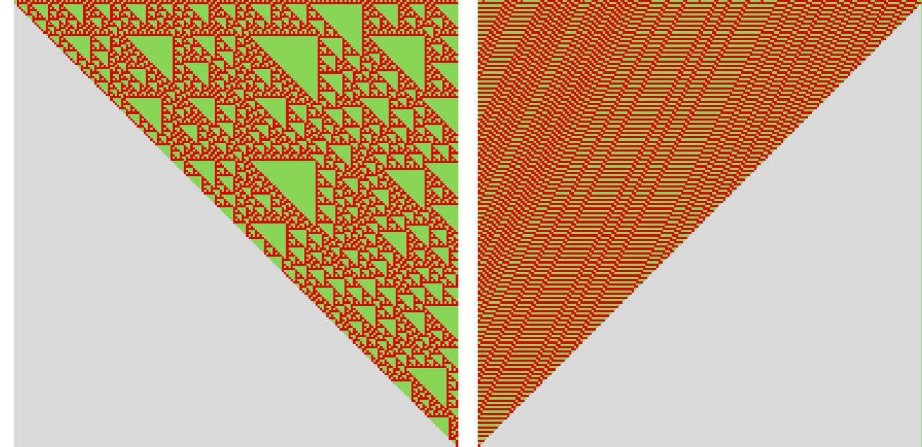
So, for example, if our two competing cellular automata have rules
then the successive steps in running them against each other give
where in our pictures everything about the second rule has been reversed. The actions taken on each step can now be read off either from the opponent initial conditions, or from the outer diagonals of the final pattern generated:
To analyze “competition” between rules we can assign payoffs, say from the match-or-not game:
And in this case we get the following cumulative payoffs:
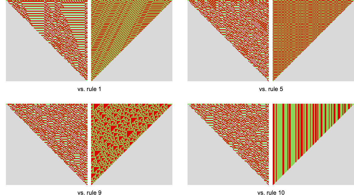
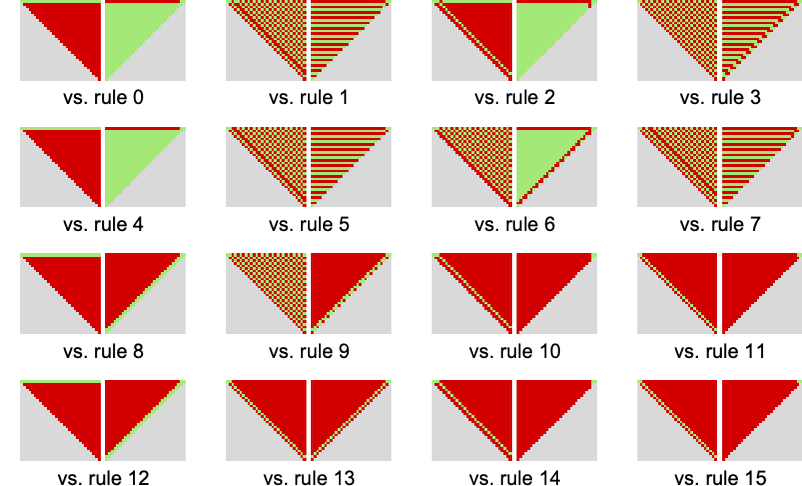
There are altogether 16 possible cellular automaton rules of the kind we’re using here:
Running each one against every other we get the following array of limiting mean payoffs:
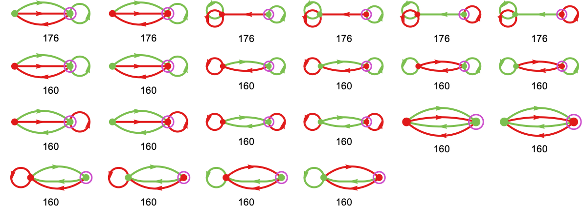
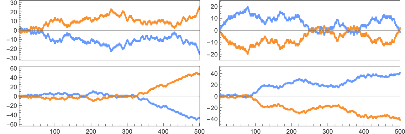
Some notable “competitions” include:
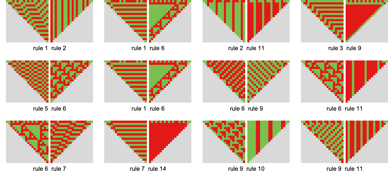
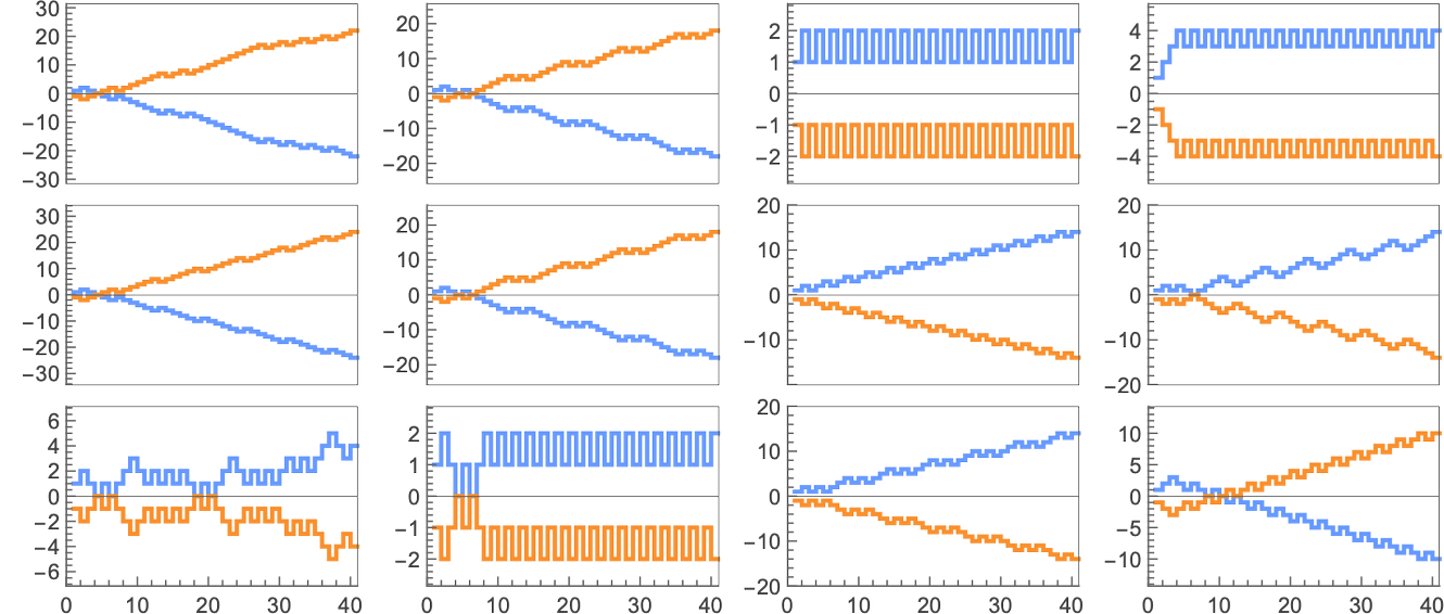
The cumulative mean (match-or-not) payoffs in these cases are:
For most of these pairs of rules the winner quickly becomes clear. But for the case of rule 6 vs. rule 7 it’s more complicated—and after 500 steps it’s still not at all clear which rule will win:
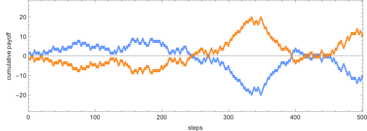
The underlying behavior is:
On their own, these two rules behave in rather simple ways (indeed, rule 7 is just XOR):
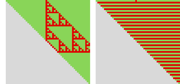
But when they’re set up in competition, the effective rule that emerges has much more complex—and apparently unpredictable—behavior, with no sign, for example, of periodicity.
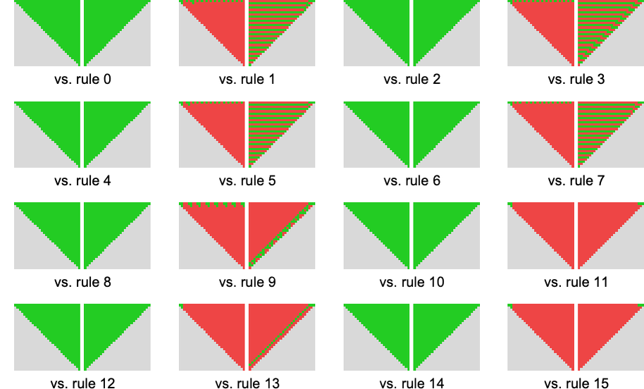
Looking across all the rules, the one with the largest average mean payoff turns out to be rule 14:
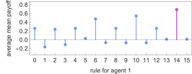
In a sense, rule 14 finds a very “simple solution”, generating either constant or period-2 behavior, and forcing its opponent to do likewise—and in the end giving an average mean payoff of exactly –![]() ≈ –0.69:
≈ –0.69:
What about with more complicated cellular automaton rules? Are the winners still ones with simple behavior?
Let’s look at the 3-color analogs of our cellular automaton rules. There are 332 = 19683 of these. And in each case we can “make a decision about the next action” by looking at the final value mod 2. Running all these rules against the 16 2-color rules the distribution of scores is:
And once again the best-performing rules (such as rule 15911) behave in rather simple ways:
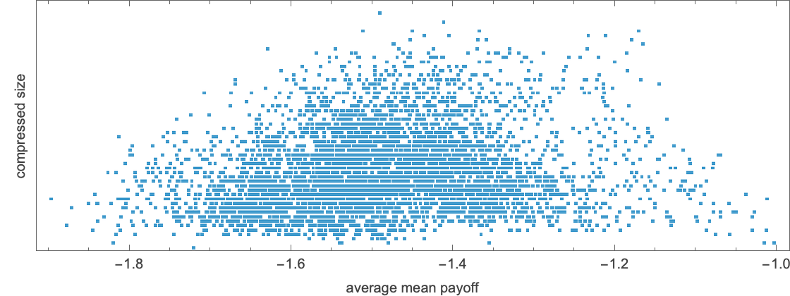
Looking—as we did for finite state machines—at the compressed size of patterns versus the average mean payoff in the corresponding competition
we see that the highest payoff rules tend to behave in simpler ways.
The rules with the most complicated behavior (at least by this measure) have average mean payoffs near zero. A typical example is rule 11948:
Some of the more complicated competitions in this case are:
What about different games with different payoffs? The underlying behavior of particular rules competing with each other will always be the same. But their payoffs will be different. And so, for example, in prisoner’s dilemma, the cumulative payoffs for 2-color rule 6 vs. 2-color rule 7 are now:
Playing each 2-color rule against all others the average mean payoffs obtained are:
Rule 13 has the highest average mean payoff (of –1), and shows fairly simple behavior:
Looking at compressed size versus average mean payoff for games between 3-color and 2-color rules, the phenomenon of high payoff being associated with simpler behavior seems even more marked for prisoner’s dilemma than for match-or-not:
We’ve looked at finite state machines competing with finite state machines, and cellular automata competing with cellular automata. But what about cellular automata competing with finite state machines?
Here’s an example of a particular step in a competition between a cellular automaton and a finite state machine
and here are the cumulative payoffs in this case for the match-or-not game:
Running all 16 cellular automaton rules of this type against all 2-state finite state machines the mean payoffs are:

Averaging over all finite state machines, the mean payoffs for the possible cellular automata are:
Rather boringly, the winning cellular automaton is rule 0, which generates ![]() in response to anything any finite state machine does:
in response to anything any finite state machine does:
This yields an average mean payoff of only +0.181. But what if we use 3-color cellular automata? Here are the average mean payoffs in that case—with the winning case highlighted:
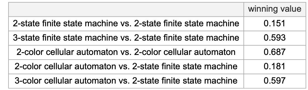
Summarizing the various competitions between different types of strategies, we see that—running against 2-state finite state machines—the most successful competitors are, by a small margin, 3-color cellular automata:
Just as we did above for finite state machines, we can consider adaptive evolution of cellular automaton rules (which is also something I’ve studied in other contexts somewhat extensively elsewhere). As a first case, let’s consider adaptively evolving a 4-color cellular automaton rule to get the best mean payoff against the most successful 3-state finite state machine above, machine 1165. At each step of adaptive evolution, we’ll randomly change one of the
The “breakthroughs” correspond to the following rules:
And as is often the case, the early breakthroughs are somewhat complicated, but in the end the “solution” that emerges shows rather simple behavior—something we can see at least some evidence for if we put the results at successive mutation steps together:
What about adapting cellular automata to compete with other cellular automata? As an example, let’s use adaptive evolution to find a 6-color cellular automaton with the largest average mean payoff when competing with all 16 of the 2-color cellular automata we’ve considered. Here’s a typical fitness curve for this case:
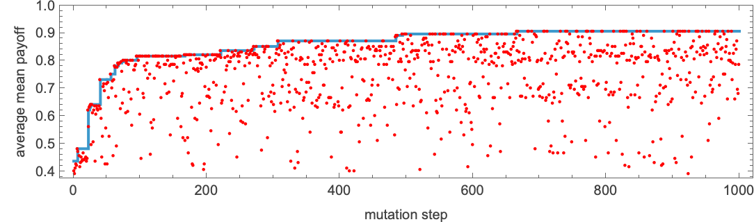
After 1000 mutation steps, it’s reached a rule that gives average mean payoff 0.91. And here’s what happens when that rule competes with all our 2-color rules:
What if (as for finite state machines above) both a rule and its opponent are undergoing adaptive evolution—say on alternating steps? Here’s an example of the successive payoffs one gets with a pair of 4-color rules:
And here are the corresponding actual behaviors:
What are the underlying cellular automata doing? Here are results at a sequence of mutation steps—illustrating that adaptive evolution can select both rules with very simple behavior and ones with somewhat more complex behavior:
We’ve looked at strategies based on finite state machines and strategies based on cellular automata. Now let’s talk about strategies based on Turing machines. For our purposes, we can think of Turing machines as in some ways interpolating between finite state machines and cellular automata—though they also introduce some entirely new features.
Our basic setup will be to use the opponent’s actions as initial values on a Turing machine tape, with the latest value on the right, which is where the Turing machine head is initially placed. We then run the Turing machine until its head goes further to the right than it’s ever gone before, at which point we determine the next action from the value that appears at the initial head position.
For example, consider a Turing machine defined by the rule:
Then imagine that the sequence of opponent actions so far is:
Running the Turing machine with this as its initial condition we get the following:
And from this we can then read off “the next move” according to our “Turing machine strategy”, in this case ![]() .
.
In our finite state machine and cellular automaton setups we did just one step of evolution for each step in our game. In our Turing machine setup, at every step in our game we’re running the Turing machine for as many steps as it takes for the head to go further to the right than it started.
Here’s what happens if we take a particular sample 3-state finite state machine
and have it compete with the Turing machine above:
With match-or-not the cumulative mean payoffs here are:
There are a total of 4096 Turing machines of the type we’re using here (with s = 2 states and k = 2 colors). Running each of these against our sample 3-state machine the mean payoffs in the match-or-not game for all the Turing machines are:
There are several Turing machines that have limiting mean payoffs of +1. An example is machine 2529:
There’s a tricky issue that comes up here, though. Our Turing machine strategy works by running a Turing machine until its head goes further to the right than it started—so that we can consider that it halts. But what if it never halts, as in:
For our purposes we’re just saying that in this case, the payoff is undefined. And if such an undefined payoff ever occurs in a particular game, we assume the mean payoff for the whole game is undefined—leaving a gap in the plot above.
What if we have Turing machines compete against, say, all distinct 2-state finite state machines? Here are the average mean payoffs in that case (the gaps are for machines that don’t halt):
The maximum of +0.4 is achieved for Turing machine 2403
which yields the following behaviors and limiting payoffs when
competing with each of the 22 distinct 2-state finite state machines:
So what about Turing machines competing with Turing machines? To keep things manageable, we can look at 1-state Turing machines, of which there are only 16 (with k = 2). Running each of these machines against each other, the array of mean payoffs is (the gray entries correspond to cases where one of the Turing machines doesn’t halt):
The average mean payoff for each of these machines is given by:
The “winner” among the machines is Turing machine 13:
Running this machine against all other s = 1, k = 2 Turing machines the behaviors we get are:
If we look at the cumulative payoffs, we see that many give mean payoffs that approach 1, though some do not, yielding in the end an average mean payoff of about +0.81:
A typical competition between 2-state Turing machines is
which yields a slightly more complicated pattern of cumulative payoffs:
What happens if 2-state and 1-state Turing machines compete? Here’s the array of mean payoffs for all 4096 2-state machines running against the 16 1-state machines:

The average mean payoffs for 2-state machines are as follows—again with maximum 0.81:
We’ve now seen many examples of the ruliology of competition. And, perhaps more than anything else, it’s now clear that if we look—ruliologically—at all possible programs of particular types, the picture of how competition works is quite complicated, even when all the programs involved are simple.
In a sense, this is a typical result of computational irreducibility: to know how competitions between programs will work out, there’s basically no choice but to run them and see what happens.
Sometimes the programs that win do so in very simple ways—in effect “exploiting simple hacks”. But in other cases, things are more complicated. Sometimes two competing programs with both show complex behavior, and in a sense, it’ll “just so happen” that one of them wins. But sometimes the win will be more systematic. And typically this happens because the behavior effectively plugs into some pocket of computational reducibility that systematically out-competes opponents of a certain type.
We’ve mostly looked at extremely simple programs which in some sense inevitably have to “expose the same rules” to every competitor. But particularly if we have a fairly small collection of competitors, a sufficiently large program can in effect expose a different part of its rules for different competitors, and so have a “customized substrategy” that separately wins against different possible competitors.
In looking at adaptive evolution of strategies we’ve often dealt with larger programs. And we’ve typically seen that the adaptive evolution can be quite successful at finding winning strategies. But—as is typically the case with adaptive evolution—there’s no obvious way to “describe the mechanism” of the strategies that are produced. Instead, it’s more like what we’ve seen in other studies of adaptive evolution: the process of evolution puts together certain “lumps of irreducible computation” that in our case here in effect “just happen” to be competitively successful.
Different games—corresponding to different patterns of payoffs—lead to results that are different in detail. And if one constructs a detailed narrative about the course of a game, it may well seem different for different games. But at an overall level, there seems to be remarkable similarity between different games—and the key phenomena seem very much the same.
What does this all say about practical situations where there’s competition between agents? One thing is that it’s typically going to be difficult to “predict in advance” or “prove a theorem” about what the best strategy will be. There’s enough computational irreducibility that one will basically just have to try running different competitions and seeing what happens. And in a sense the very diversity of behavior we’ve seen here supports the idea that ruliological investigation is critical. Finding some simple parametrization of possible strategies won’t be enough to get an accurate sense of everything that can happen. There’s no choice but to systematically enumerate some version of “all computationally possible strategies”. Which is what we can do in our ruliological investigations.
And, yes, what we’ve done here just scratches the surface of studying the ruliology of competition. For a start, one can scale up the size of the programs, and see what new phenomena occur. One can expect that mostly things will be the same—with computational irreducibility the dominant force. But there may be new and unexpected pockets of reducibility, perhaps each with their own “paths to competitive success”.
One can also imagine investigating different kinds of computational systems—that serve as metamodels appropriate for different applications. The Principle of Computational Equivalence suggests that there’ll be a certain universality to the overall results. But details will be different. And those details will potentially be important, particularly in interpreting results for very different domains. Even if what matters for ultimate purposes of competition is well captured by finite state machines—or a cellular automata—the way one gets to these from microscopic biology, human decision making, societal interactions, AI competition, etc. may be very different.
There’s a long history to formal studies of games—and indeed early developments in areas like combinatorics and probability were largely driven by them. The modern field known as game theory emerged in the 1940s, concentrating on the question of optimal strategies given particular patterns of payoffs. Most often the idea is to analyze what happens when each player makes a single move—albeit perhaps a probabilistic one, with averages taken over many instances. Fairly complete (though sometimes complicated) mathematical results have been derived for this kind of setup (and are now, for example, implemented in the Wolfram Language). But what about repeated, or iterated, games of the kind we’ve been discussing here? In the early days of game theory there was discussion about defining strategies as arbitrary mappings from histories to actions—and various rather abstract mathematical results were proved, particularly for applications in economics.
But by the 1970s there started to emerge the idea that one should model agents as having “bounded rationality”, and corresponding to limited computational systems. And by the end of the 1970s computer experiments were being done on competition between what amounted to simple programs. A notable example was the tournament organized by Bob Axelrod for the prisoner’s dilemma game. In this tournament, a collection of particular programs were submitted by different individuals, and run against each other. The conclusion was that the “tit for tat” strategy (that can be thought of as a finite state machine) came out best—a result from which much has been made about the value of cooperation, etc.
I must admit that I was always suspicious of the result. It seemed very unscientific to have just looked at programs people happened to have submitted for the tournament. Why not instead systematically enumerate all possible programs and see what happens? In my own work—starting at the beginning of the 1980s—I was routinely doing this kind of thing, particularly for cellular automata. I always found the setup for game theory a little arbitrary, and fiddly, and I was discovering more than I could keep up with just investigating the behavior of individual programs, without trying to have them compete with each other. Still, finally, in the mid-1990s, I did have a look at what happens when a range of possible programs (in that case, cellular automata) compete with each other. I summarized the result in a small note at the end of my book A New Kind of Science:

I always meant to come back and look at this in more detail. And finally my recent work in the foundations of biological evolution made me think it was time to do it. I found out that there was some literature on using models like finite state machines as strategies for iterated games. But so far as I could tell, the kind of systematic ruliological investigation I had imagined had never been done. Which is why I recently decided it was finally time to do it…
Thanks to Willem Nielsen, Brian Ashiundu and Júlia Campolim of the Wolfram Institute for their extensive help. Several participants at our summer programs have done projects about games between programs that I’ve suggested: Rodrigo Bazaes, Kantaporn Danchaivijitr and Aziz Sahibnazarov. Over the course of many years, I’ve discussed game theory and related ideas with quite a few people, including Brian Arthur, Bob Axelrod, Seth Chandler, Roger Germundsson, Paul Harrald, Jozsef Konczer, Pedro Marquez-Zacarias, Eric Maskin, Zsombor Méder, Chrystopher Nehaniv, Scott Page, Jordan Pollack, John Maynard Smith, Stan Reiter, Nassim Taleb, Valeriu Ungureanu and Marc Vicuna. (Notable game theorist John Nash was a long-time user of what’s now Wolfram Language, and attended conferences about it, but I never personally met him.)
2026-02-24 05:52:54
![]()
LLMs don’t—and can’t—do everything. What they do is very impressive—and useful. It’s broad. And in many ways it’s human-like. But it’s not precise. And in the end it’s not about deep computation.
So how can we supplement LLM foundation models? We need a foundation tool: a tool that’s broad and general and does what LLMs themselves don’t: provides deep computation and precise knowledge.
And, conveniently enough, that’s exactly what I’ve been building for the past 40 years! My goal with Wolfram Language has always been to make everything we can about the world computable. To bring together in a coherent and unified way the algorithms, the methods and the data to do precise computation whenever it’s possible. It’s been a huge undertaking, but I think it’s fair to say it’s been a hugely successful one—that’s fueled countless discoveries and inventions (including my own) across a remarkable range of areas of science, technology and beyond.
But now it’s not just humans who can take advantage of this technology; it’s AIs—and in particular LLMs—as well. LLM foundation models are powerful. But LLM foundation models with our foundation tool are even more so. And with the maturing of LLMs we’re finally now in a position to provide to LLMs access to Wolfram tech in a standard, general way.
It is, I believe, an important moment of convergence. My concept over the decades has been to build very broad and general technology—which is now a perfect fit for the breadth of LLM foundation models. LLMs can call specific specialized tools, and that will be useful for plenty of specific specialized purposes. But what Wolfram Language uniquely represents is a general tool—with general access to the great power that precise computation and knowledge bring.
But there’s actually also much more. I designed Wolfram Language from the beginning to be a powerful medium not only for doing computation but also for representing and thinking about things computationally. I’d always assumed I was doing this for humans. But it now turns out that AIs need the same things—and that Wolfram Language provides the perfect medium for AIs to “think” and “reason” computationally.
There’s another point as well. In its effort to make as much as possible computable, Wolfram Language not only has an immense amount inside, but also provides a uniquely unified hub for connecting to other systems and services. And that’s part of why it’s now possible to make such an effective connection between LLM foundation models and the foundation tool that is the Wolfram Language.
On January 9, 2023, just weeks after ChatGPT burst onto the scene, I posted a piece entitled “Wolfram|Alpha as the Way to Bring Computational Knowledge Superpowers to ChatGPT”. Two months later we released the first Wolfram plugin for ChatGPT (and in between I wrote what quickly became a rather popular little book entitled What Is ChatGPT Doing … and Why Does It Work?). The plugin was a modest but good start. But at the time LLMs and the ecosystem around them weren’t really ready for the bigger story.
Would LLMs even in the end need tools at all? Or—despite the fundamental issues that seemed at least to me scientifically rather clear right from the start—would LLMs somehow magically find a way to do deep computation themselves? Or to guarantee to get precise, reliable results? And even if LLMs were going to use tools, how would that process be engineered, and what would the deployment model for it be?
Three years have now passed, and much has clarified. The core capabilities of LLMs have come into better focus (even though there’s a lot we still don’t know scientifically about them). And it’s become much clearer that—at least for the modalities LLMs currently address—most of the growth in their practical value is going to have to do with how they are harnessed and connected. And this understanding highlights more than ever the broad importance of providing LLMs with the foundation tool that our technology represents.
And the good news is that there are now streamlined ways to do this—using protocols and methods that have emerged around LLMs, and using new technology that we’ve developed. The tighter the integration between foundation models and our foundation tool, the more powerful the combination will be. Ultimately it’ll be a story of aligning the pre-training and core engineering of LLMs with our foundation tool. But an approach that’s immediately and broadly applicable today—and for which we’re releasing several new products—is based on what we call computation-augmented generation, or CAG.
The key idea of CAG is to inject in real time capabilities from our foundation tool into the stream of content that LLMs generate. In traditional retrieval-augmented generation, or RAG, one is injecting content that has been retrieved from existing documents. CAG is like an infinite extension of RAG, in which an infinite amount of content can be generated on the fly—using computation—to feed to an LLM. Internally, CAG is a somewhat complex piece of technology that has taken a long time for us to develop. But in its deployment it’s something that we’ve made easy to integrate into existing LLM-related systems and workflows. And today we’re launching it, so that going forward any LLM system—and LLM foundation model—can count on being able to access our foundation tool, and being able to supplement their capabilities with the superpower of precise, deep computation and knowledge.
Today we’re launching three primary methods for accessing our Foundation Tool, all based on computation-augmented generation (CAG), and all leveraging our rather huge software engineering technology stack.
![]() Immediately call our Foundation Tool from within any MCP-compatible LLM-based system. Most consumer LLM-based systems now support MCP, making this extremely easy to set up. Our main MCP Service is a web API, but there’s also a version that can use a local Wolfram Engine.
Immediately call our Foundation Tool from within any MCP-compatible LLM-based system. Most consumer LLM-based systems now support MCP, making this extremely easy to set up. Our main MCP Service is a web API, but there’s also a version that can use a local Wolfram Engine.
![]() A one-stop-shop “universal agent” combining an LLM foundation model with our Foundation Tool. Set up as a drop-in replacement for traditional LLM APIs.
A one-stop-shop “universal agent” combining an LLM foundation model with our Foundation Tool. Set up as a drop-in replacement for traditional LLM APIs.
![]() Direct fine-grained access to Wolfram tech for LLM systems, supporting optimized, custom integration into LLM systems of any scale. (All Wolfram tech is available in both hosted and on-premise form.)
Direct fine-grained access to Wolfram tech for LLM systems, supporting optimized, custom integration into LLM systems of any scale. (All Wolfram tech is available in both hosted and on-premise form.)
![]() Wolfram Foundation Tool Capabilities Listing »
Wolfram Foundation Tool Capabilities Listing »
For further information on access and integration options, contact our Partnerships group »
2026-02-05 04:24:57
![]()
The Wolfram Institute recently received a grant from the Templeton World Charity Foundation for “Computational Metaphysics”. I wrote this piece in part as a launching point for discussions with experts in traditional philosophy.

“What ultimately is there?” has always been seen as a fundamental—if thorny—question for philosophy, or perhaps theology. But despite a couple of millennia of discussion, I think it’s fair to say that only modest progress has been made with it. But maybe, just maybe, this is the moment where that’s going to change—and on the basis of surprising new ideas and new results from our latest efforts in science, it’s finally going to be possible to make real progress, and in the end to build what amounts to a formal, scientific approach to metaphysics.
It all centers around the ultimate foundational construct that I call the ruliad—and how observers like us, embedded within it, must perceive it. And it’s a story of how—for observers like us—fundamental concepts like space, time, mathematics, laws of nature, and indeed, objective reality, must inevitably emerge.
Traditional philosophical thinking about metaphysical questions has often become polarized into strongly opposing views. But one of the remarkable things we’ll see here is that with what we learn from science we’ll often be able to bring together these opposing views—typically in rather unexpected ways.
I should emphasize that my goal here is to summarize what we can now say about metaphysics on the basis of our recent progress in science. It’ll be very valuable to connect this to historical positions and historical thinking in philosophy and theology—but that’s not something I’m going to attempt to do here. I should also say that I’m going to concentrate on the major intellectual arc of what one can think of as a new scientific approach to metaphysics; the technical details of the science I’ve mostly already discussed elsewhere.

We’re going to begin our journey by talking about the traditional objective of physics: to find abstract theories that describe what we observe and measure in the physical world. From the history of physics we’ve come to expect that such theories will always end up being at best successive approximations. But the new possibility raised by our Physics Project is that we may now finally have reached the end: a truly fundamental theory of physics, that provides a complete description of the lowest-level “machine code” of our universe.
Already in antiquity the question arose of whether the universe is ultimately a continuum or is made of discrete atomic elements. By the end of the nineteenth century it was finally established that matter, at least, consists of discrete elements. And soon it became clear that light could be thought of in the same way. But what about space? Ever since Euclid, it had been assumed that space was a continuum. And efforts in the early twentieth century to see whether it, like matter, might be discrete did not work out.
But a century later, building on new, computationally inspired ideas, our Physics Project starts from the concept that space is not just a simple continuum. Instead, it’s a complicated discrete structure that in fact represents every aspect of our universe—both what we normally think of as space, and everything in it. There are many ways one can imagine describing this structure. A convenient one is to say that it consists of a very large number of discrete intrinsically identical “atoms of space”—that one can think of as being like disembodied geometrical points—whose only property (other than being distinct) is how they’re abstractly related to other atoms of space. In other words, we imagine describing the whole structure of the universe in terms of the pattern of relations between the atoms of space. And it’s convenient to represent this as a hypergraph whose nodes are atoms of space, and whose hyperedges define the relations between them. (If relations are only between pairs of nodes, this becomes an ordinary graph.)
An important piece of intuition that comes from our practical experience with computers is that it’s possible to represent everything we deal with in terms of bits. But when we also want to represent the structure of space it’s better to think not in terms of bits in some predetermined arrangement, but instead in terms of the lower level and more flexible “data structure” defined by a hypergraph.
So how can the universe as we normally perceive it emerge from this? It’s very much analogous to what happens with matter. For example, even though something like water consists of discrete molecules, the aggregate effect of them is to produce seemingly continuous fluid behavior. But then—still made up of the same underlying molecules—we can have discrete eddies in the fluid, analogous in the case of space to particles like electrons (or, for that matter, black holes).

If there’s a hypergraph that’s the ultimate “data structure” of the universe, what are the algorithms that get applied to it? Just as we imagine the data structure to consist of discrete elements, so also we imagine that changes to it occur by discrete events. And for now we can imagine that there’s some fixed rule that determines these elementary events. For example, the rule might be that whenever a piece of the hypergraph has some specified form, it should be replaced by a piece of hypergraph with some other specified form.
We can think of the application of such a rule as corresponding to the computation of the “next state” of the universe from the previous one. And if the rule is repeatedly applied, it will generate a whole sequence of updated states of the universe. And we can then identify the progression of these states as corresponding to the progression of time in the universe.
It’s notable that in this setup space and time are, at least at the outset, different kinds of things. Space is associated with the structure of the hypergraph, yet time is associated with computation on it.
Still, just as the hypergraph defines relations between atoms of space, we can imagine a causal graph that defines “causal relations” between events. Any particular event can be thought of as taking some collection of atoms of space as “inputs”, and producing some other collection of atoms of space as “outputs”. But this then implies a causal relation between events: any event that uses as input an atom of space that was generated as output by another event can be thought of as “causally dependent” on that other event.
And the whole pattern of these causal relations ultimately defines a causal graph for all events in the universe—that in a sense encodes the structure of the universe in both space and time.
But given such a causal graph, can we reconstruct a series of hypergraphs from it? We can think of such hypergraphs as representing successive “instantaneous states of space”. And—just like in relativity—it turns out that there isn’t a unique possible such sequence of states. Instead, there are many different sequences, all consistent with the underlying causal graph—and corresponding in traditional physics terms to different relativistic reference frames.
In effect, therefore, we can think of the causal graph as being the “true representation” of information about the universe. Any particular “reconstructed” sequence of hypergraphs inevitably involves arbitrary choices.
When we introduced the causal graph, we talked about building it by starting from a particular hypergraph, and then looking at the effect of applying rules to it. But the point is that it turns out there’s a lot of choice in both the hypergraph and how we apply the rules, but (as a result of the phenomenon of causal invariance) essentially all choices will lead us to the same causal graph.
We might have imagined that given a fundamental theory of physics we should be able to ask what the universe in some sense “statically is”. But what we’re discovering is that we should instead be talking about the processes that happen in the universe—as represented by the causal graph.
We can identify the passage of time as the progression of events in the causal graph. But why is there even something like space? Ultimately it turns out to be a reflection of the “entanglement” of different sequences of events in the causal graph—and its structure is in effect a map of the relations between these sequences of events (a structure which can conveniently be represented by a hypergraph).
Imagine starting from one event in the causal graph, then tracing a sequence of events that depend on it. We can think of the successive events as occurring progressively later in time. But what about two events that are both immediate successors of a given event? What is their relationship? The key idea is that even though these “sibling” events occur “at the same time”, they are still separated—in what we can think of as space.
But how then is “space as a whole” formed? Ultimately it’s something very dynamic. And indeed it’s the continual occurrence of events in the universe that “knits together” the structure of space. Without such “activity”, there would be nothing we could coherently consider as “space”.
At the level of atoms of space there is nothing permanent in the universe; in every elementary event, atoms of space are destroyed, and new ones created. But somehow at an aggregate level there is a certain stability to what emerges. It’s again a little like with fluids, where the microscopic motions of huge numbers of underlying molecules lead in the aggregate to the laws of fluid mechanics.
But what then are the aggregate laws that emerge from large numbers of hypergraph updates? Remarkably enough, they almost inevitably turn out to be exactly the Einstein equations: the equations that seem to govern the large-scale structure of spacetime. So even though what’s “there underneath” is just what we might think of as “abstract” atoms of space and rules for rewriting relations between them, what emerges is something that reproduces familiar elements of what we think of as “physical reality”.

If there’s a rule that can ultimately reproduce the behavior of the universe, how complicated a rule does that need to be? Our traditional intuition—say from experience from engineering—is that one needs a complicated rule if one wants to produce complicated behavior. But my big discovery from the early 1980s is that this isn’t the case—and that in fact it’s perfectly possible even for extremely simple underlying rules (like my favorite “rule 30”) to produce behavior of immense complexity.
But why ultimately does this happen? We can think of running a rule as being like running a program, or, in other words, like doing a computation. But how sophisticated is that computation? We might have thought that different rules would do incomparably different computations. But the existence of universal computation—discovered a century ago—implies that in fact there’s a class of universal rules that can effectively emulate any other rule (and this is why, for example, software is possible).
But actually there’s a lot more that can be said. And in particular my Principle of Computational Equivalence implies that essentially whenever one sees a system whose behavior is not obviously simple, the system will actually be doing a computation that is in some sense as sophisticated as it can be. In other words, sophisticated computation isn’t just a feature of specially set up “computer-like” systems; it’s ubiquitous, even among systems with simple underlying rules.
So what does this mean? It’s often considered a goal of science to be able to predict what systems will do. But to make such a prediction requires in a sense being able to “jump ahead” of the behavior of the system itself. But the Principle of Computational Equivalence tells us that this won’t in general be possible—because it’s ubiquitous for the system we’re trying to predict to be just as computationally sophisticated as the system we’re trying to use to predict it. And the result of this is the phenomenon of computational irreducibility.
You can always find out what a system will do just by explicitly running its rules step by step. But if the system is computationally irreducible there’ll be no general way to shortcut this, and to find the result with reduced computational effort.
Computational irreducibility is what irreducibly separates underlying rules from the behavior they produce. And it’s what causes even simple rules to be able to generate behavior that cannot be “decoded” except by irreducibly great computational effort—and therefore will be considered random by an observer with bounded computational capabilities.
Computational irreducibility is also what in a sense makes time something “real”. We discussed above that the passage of time corresponds to the progressive application of computational rules. Computational irreducibility is what makes that process “add up to something”. And the Principle of Computational Equivalence is what tells us that there’s something we can think of as time that is in effect “pure, irreducible computation” independent of the system in which we’re studying it.
It’s very much the same story with space. Computational irreducibility in general leads to a certain “uniform effective randomness” in the structure of hypergraphs, which is what allows us to imagine that there’s a definite “substrate independent” concept of space.
There’s a close analogy here to what happens in something like a fluid. At a molecular level there are lots of molecular collisions going on. But the point is that this is a computationally irreducible process—whose end result is enough “uniform effective randomness” that we can meaningfully talk about the properties of the fluid “in bulk”, as a thing in itself, without having to mention that it’s made of molecules.
So how does all this relate to our original metaphysical question of what there ultimately is? Computational irreducibility introduces the idea that there’s something robust and invariant about “pure computation”—something that doesn’t depend on the details of what’s “implementing” that computation. Or, in other words, that there’s a sense in which it’s meaningful to talk about things simply being “made of computation”.

In talking about things like a hypergraph representing space and everything in it, we’re giving in a sense an objective description of the universe “from the outside”. But what ultimately matters to us is not what’s “in principle out there”, but rather what we actually perceive. And indeed we can think of science as being first and foremost a way to find narrative descriptions which fit in our minds of certain aspects of what’s out there.
But given computational irreducibility, why is this even possible? Why are there ever, for example, “laws of nature” which let us make predictions about things, even with the bounded amount of computation that our finite minds can do?
The answer is related to an inevitable and fundamental feature of computational irreducibility: that within any computationally irreducible process there must always be an infinite number of pockets of computational reducibility. In other words, even though computational irreducibility makes it irreducibly difficult to say everything about what a system will do, there will always be pockets of reducibility which allow one to say certain things about it. And it’s such pockets of reducibility that our processes of perception—and our science—make use of.
Once again we can use fluid dynamics as an example. Even though the detailed pattern of underlying molecular motions in a fluid is computationally irreducible, there are still computationally simple overall laws of fluid flow—that we can think of as being associated with pockets of computational reducibility. And from our point of view as computationally bounded observers, we tend to think of these as the laws of the fluid.
In other words, the laws we attribute to a system depend on our capabilities as observers. Consider the Second Law of thermodynamics, and imagine starting from some simple configuration, say of gas molecules. The dynamics of these molecules will generically correspond to a computationally irreducible process—whose outcome to a computationally bounded observer like us will seem “increasingly random”. Of course, if we were not computationally bounded, then we’d be able to “decode” the whole underlying computationally irreducible process, and we wouldn’t believe in the presence of seemingly increasing randomness, or, for that matter, the Second Law. But—regardless of any details—as soon as we’re computationally bounded, we’ll immediately perceive the Second Law.
We might have assumed that the Second Law was some kind of intrinsic law of nature—directly related to what there ultimately is. But what we see is that the Second Law is something that emerges because of us, and our characteristics as observers, and in particular our computational boundedness.
There are other things that also work this way—for example, our belief in a coherent notion of space. At the lowest level we imagine that there’s a discrete hypergraph being updated through what’s ultimately a computationally irreducible process. But as computationally bounded observers we only perceive certain aggregate features—that correspond in effect to a pocket of computational reducibility associated with our simple, continuous perception of space.
When we think about spacetime—and for example about deriving its relativistic properties—there’s another feature of us as observers that also turns out to be important: the fact that we assume that we are persistent in time, and that—even though we might be made of different atoms of space at every successive moment of time—we can still successfully knit together perceptions at successive moments of time to form a single thread of experience. In a sense this is a “simplification” forced upon us by our computational boundedness. But it’s also in many ways at the core of what we think of as our notion of consciousness (which is something I’ve written about at some length elsewhere).
The Principle of Computational Equivalence implies that sophisticated computation is ubiquitous—and certainly not something special to brains. And indeed it seems that brains actually concentrate on a specific—and in many ways limited—form of computation. They take in large amounts of sensory data, and in effect compress it to derive what’s ultimately a thin stream of actions for us to take. At a biological level, there’s always all sorts of activity going on across the billions of neurons in our brains. But our brains are, it seems, specially constructed to concentrate all that activity down to what’s essentially a single thread of thought, action and “experience”. And it’s the fact that this is a single thread that seems to give us our sense of coherent existence, and in effect, of consciousness.

Traditional classical physics talks about definite things happening in the universe—say a projectile following a definite path, determined by its laws of motion. But quantum mechanics instead talks about many paths being followed—specifying only probabilities for their various outcomes.
In this history of physics quantum mechanics was a kind of “add on”. But in our Physics Project it’s immediately essential, and unavoidable. Because the rules that we define simply say that whenever there is a piece of a hypergraph that matches a particular pattern, it should be transformed. But in general there will be many such matches—each one producing a different transformation, and each one in effect initiating what we can think of as a different path of history. And in addition to such branching, there can also be merging—when different transformations end up producing the same hypergraph.
We can represent all these branching and merging paths of history by what I call a multiway graph. And we can think of such a multiway graph as giving a complete description of “what happens” in the universe.
But as we discussed above, observers like us maintain just a single thread of experience. And that means we can’t directly perceive a whole multiway graph. Instead, we have to effectively pick out just one path from it. But which path will it be? At the level of the formalism of quantum mechanics—or of our Physics Project—the only thing we talk about is the whole collection of all paths. So something else must determine the path.
In physical space, we’re used to the idea that we as observers are localized at a particular position, and only get to directly perceive what’s around where we are. Across all of physical space, there are lots of things going on. But because of where we happen to be, we only get to directly perceive a tiny sample of them.
So is something similar going on in picking paths of history from the multiway graph? It seems that it is. If we take a slice across the multiway graph at any particular time, we’ll have lots of “dangling ends” of paths of history, each associated with a different state of the universe. But inevitably there are lots of relations between these states. (For example, two states might have an immediate common ancestor.) And it turns out that we can think of the states as being laid out in what we can call “branchial space”.
And just like in physical space, we can expect that we as observers are localized in branchial space. So that means that even though there are at some level many different paths of history, we only get to perceive ones that are around “where we are”. And just like there’s no “theory” that tells us where we find ourselves in physical space (which planet, which galaxy, etc.), the same is true in branchial space. One day we might have some way to describe our location in branchial space, but for now the best we can do is say that it’s “random”.
And this, I believe, is why outcomes in quantum mechanics seem to us random. The whole multiway graph is completely determined (as wave functions etc. are even in the standard formalism of quantum mechanics). But which part of the multiway graph we as observers sample depends on where we are in branchial space.
And we can expect that just as we humans are all close together in physical space, so are we in branchial space. And this means that even though in the abstract the result of, say, some particular quantum measurement might seem “random”, all human observers—being nearby in branchial space—will tend to agree what that result is, and at least among them, there’ll be something they can consider “objective reality”.

The remarkable implication of our Physics Project is that our whole universe, in all its richness, can emerge just from the repeated application of a simple underlying rule. But which rule? How would it be selected?
The idea of the ruliad is to imagine that no selection is needed—because all rules are being used. And the ruliad is what comes out: the entangled limit of all possible computational processes.
We discussed in the context of quantum mechanics the idea that a given rule can get applied in multiple ways, leading to multiple paths of history. The ruliad takes this idea to the limit, applying not just one rule in all possible ways, but all possible rules in all possible ways.
We can imagine representing the ruliad by a giant multiway graph—in which there is a path that represents any conceivable specific computation. And what fundamentally gives the ruliad structure is that these paths can not only branch but also merge—with mergers happening when different states lead to equivalent outcomes which are merged in the multiway graph.
At first we can think of the ruliad as being built from all possible hypergraph rules in our Physics Project. But the Principle of Computational Equivalence implies that actually we can use any type of rule as our basis: since the ruliad contains all possible computational processes its final form will be the same.
In other words, however we end up representing it, the intrinsic form of the ruliad is still the same. Once we have the concept of computation (or of following rules), the ruliad is an inevitable consequence. In some sense it is the ultimate closure of the concept of computation: the unique object that encapsulates all possible computational processes and the inevitable relations between them.
We got to the ruliad by thinking about physics, and about the ultimate infrastructure of our physical universe. But the ruliad is something much more general than that. It’s an abstract object that captures everything that is computationally formalizable, along with the elaborate structure of relations between such things.
Of course, the idea that the ruliad can describe our actual physical universe is ultimately just a hypothesis—though one that’s strongly encouraged by the success of our Physics Project.
How could it be wrong? Well, our universe could involve hypercomputation—which is not finitely captured by the ruliad. And we might have to consider a whole hierarchy of possible hyperruliads. (Though as we’ll see, any effects from this would likely be beyond anything observers like us could perceive.)
But assuming that the ruliad is the ultimate infrastructure for everything we can then ask what it’s made of. At some level we could just say it’s made of abstract computational processes. But what are those processes operating on? Again, abstract things. But we can imagine decomposing those abstract things. And while inevitably there will be different ways to do this, it’ll often be convenient to imagine that they consist of relations between ultimate, indivisible objects—which we can describe as “atoms of existence”, or what I’ve called “emes”.
In our Physics Project, we identified emes with atoms of space. But in talking about the ruliad in general, we can think of them just as the “ultimate raw material for existence”. Emes have no structure of their own. And indeed the only intrinsic thing one can say about them is that they are distinct: in a sense they are elementary units of identity. And we can then think of it being the relations between them that build up the ruliad—and everything it underlies.

Our original metaphysical question was: “What ultimately is there?” And at some level our science has now led us to an answer: the ruliad is everything there ultimately is.
But what about what there is for us? In other words, what about what there ultimately is in what we perceive and experience? Inevitably, we as observers must be part of the ruliad. And our “inner experiences” must similarly be represented within the ruliad. But in and of itself that’s not enough to tell us much about what those experiences might be. And we might imagine that to work this out, we’d need to know a lot of the particular details of our construction, and our place in the ruliad.
But what’s emerged in the last few years is that in many important ways, we don’t. And instead just knowing certain coarse features of us as observers already implies a lot about what we must experience. In particular, if we assume that we are observers who are computationally bounded, and believe we are persistent in time, then we argue that it is inevitable that we must perceive certain laws to be operating—and those laws turn out to be exactly the three central laws of twentieth century physics: general relativity, quantum mechanics, and the Second Law of thermodynamics.
It’s a remarkable claim: the laws of physics we observe don’t just happen to be the way they are; they are inevitable for observers with the general characteristics we have. At the level of the underlying ruliad the laws of physics that we might observe are not determined. But as soon as we know something about what we’re like as observers, then we necessarily end up with our familiar laws of physics.
In a sense, therefore, the laws of physics that we experience are the way they are because we are observers that are the way we are. We already discussed this above in the case of the Second Law. And although we don’t yet know all the details, the basic conclusion is that by combining the abstract structure of the ruliad with our assumptions about what we’re like as observers, we are able to derive all three of the familiar core laws of physics from the twentieth century.
It’s worth emphasizing that what we can immediately derive are in a sense “general laws”. We know that spacetime has a certain overall structure, and its dynamics satisfy the Einstein equations. But we don’t, for example, know why the universe as we perceive it has (at least approximately) 3 dimensions of space—though my guess is that many such features of observed physics can ultimately be traced to features of the way we are as observers.
So what about observers not like us? They’re still part of the ruliad. But in a sense they’re sampling it in a different way. And they’ll potentially perceive quite different laws of physics.
It’s a very fundamental observation about our universe that we perceive it to follow fairly simple laws. But in a sense this too is just a feature of our nature as observers. Because given our computational boundedness we couldn’t really make use of—or even identify—any laws that were not in some sense simple.
The fact that simple laws are possible can be viewed as a reflection of the inevitable presence of pockets of computational reducibility within any computationally irreducible process. But it’s our computational boundedness as observers that causes us to pick them out. If we were not computationally bounded then we could operate at the level of raw computational irreducibility, and any need to pick out simple laws.
At the outset, we might have imagined that the laws of physics would somehow fundamentally be at the root of the question of “what ultimately is there?” But what we’re seeing is that actually these laws are in a sense higher-level constructs, whose form depends on our characteristics as observers. And to get to our original metaphysical question, we have to “drill down” beyond our perceived laws of physics to their “computational infrastructure”, and ultimately all the way to the ruliad.

When we ask what there ultimately is, we’re in some sense implicitly assuming that there actually is something definite—or in effect that there’s a single ultimate “objective reality”. But is that actually how things work, or does every observer, for example, in effect “have their own reality”?
In our approach, there’s a quite nuanced answer. At the very lowest level there is a single ultimate objective reality that knits everything together—and it’s the ruliad. But meanwhile, different observers can in principle experience different things. But as soon as we’re dealing with observers even vaguely like us (in the sense that they share our computational boundedness, and our belief in our own persistence) we’ve argued that it’s inevitable that they’ll always experience the core laws of physics as we know them. In other words, these laws in effect represent a single objective reality—at least across observers even vaguely like us.
But what about more detailed features of our experience? No doubt some we’ll be able to “objectively derive” on the basis of characteristics we identify as shared across all “observers like us”. But at some level, different observers will always have different experiences—not least because, for example, they are typically operating at different places in space, and indeed in general at different places in the ruliad.
Still, our everyday impression is that even though the detailed experiences, say, of different people looking at the same scene may be different, those experiences can nevertheless reasonably be thought of as all derived from the same “underlying objective reality”. So why is this? Essentially I think it’s because human observers are all very nearby in the ruliad—so they’re in a sense all sampling the same tiny part of the ruliad.
Observers at different places in the ruliad in effect sample different threads of history, that operate according to different rules. But the Principle of Computational Equivalence tells us that—just as it’s always possible to translate from one universal computational system to another—it’ll always in the end be possible to translate between what observers get by sampling at different places in the ruliad.
The difficulty of translation depends, though, on how far one is trying to go in the ruliad. Human minds exposed to similar knowledge, culture, etc. are nearby and fairly easy to translate between. Animal minds are further away, and more difficult to translate to. And when it comes to something like the weather, then even though in principle it’s computationally equivalent, the distance one has to go in the ruliad to reach it is sufficiently great that translation is very difficult.
Translation between places in the ruliad is in a sense just a generalization of translation in physical space. And the process of moving in physical space is what we describe as motion. But what actually is motion? In effect it’s having something move to a different place in space while still “being the same thing”. In our Physics Project, though, something must be made of different atoms of space if it’s at a different place in space. But somehow there must be some pattern of atoms of space that—a bit like an eddy in a fluid—one can say represents “the same thing” at different places in space.
And potentially one can think of particles—like electrons or photons—as being in a sense “elementary carriers of pure motion”: minimal objects that can move without changing.
But how does this work more generally in the ruliad? What is it that can “move” between observers, or between minds, without changing? Essentially it seems to be concepts (often in basic form represented by words). Within for example one human brain a thought corresponds to some complicated pattern of neural activity. But what allows it to be “moved” to another brain is “packaging it up” into a “concept” that can be unpacked by another brain. And at some level it’s this kind of communication that “aligns observers” to have similar inner experiences—to the point where they can be viewed as reflecting a common objective reality.
But all of this somehow presupposes that there are many observers—whose experiences can be thought of as “triangulating” to a common objective reality. If there were just one observer, though, there’s no triangulation to do, and one might imagine that all that would matter is the inner experience of that one observer.
So in a sense the very notion that we can usefully talk about objective reality is a consequence of there being many similar observers. And of course in the specific case of us humans there are indeed billions of us.
But from a fundamental point of view, why should there be many similar observers, or even any observers at all? As we discussed above, the core abstract characteristic of an observer is its ability to equivalence many possible inputs to produce a small set of possible outputs. And—although we don’t yet know how to do it—we can imagine that it would be possible to derive the fact that there must be a certain density of structures that do this within the ruliad. Could there inevitably be enough similar observers to be able to reasonably triangulate to an objective reality?
If we take the example of biology (or modern technology) it seems like what’s critical in generating large numbers of similar observers is some form of replication. And so, surprising as it might seem for something as apparently fundamental as this, it appears that our impression of the existence of objective reality is actually intimately tied up with the rather practical biological phenomenon of self replication.
OK, so what should we in the end think about objective reality? We might have imagined that having a scientific theory of the universe would immediately imply a certain objective reality. And indeed at the level of the ruliad that’s true. But what we’ve seen is that even to get our familiar laws of physics we need an observer “parsing” the raw ruliad. In other words, without the observer we can’t even talk about fundamental concepts in physics. But the point is that for a very wide range of observers even vaguely like us, many details of the observer don’t matter; certain things—like core laws of physics—inevitably and “objectively” emerge.
But the laws of physics don’t determine everything an observer perceives. Some things are inevitably determined by the particular circumstances of the observer: their position in space, in the ruliad, etc. But now the point is that observers—like us humans—are nearby enough in space, the ruliad, etc. that our perceptions will be to a large extent aligned, so that we can again usefully attribute them to what we can think of as an external objective reality.

In thinking about what there ultimately is, an obvious question is whether whatever there is has always been there—and will always be—or whether instead there’s in effect a beginning—and end—to time.
As we discussed above, in our computational paradigm, the passage of time is associated with the progressive computation of successive states of the universe. But the important point is that these states embody everything—including any potential observers. So there can never be a situation where an observer could say “the universe hasn’t started yet”—because if the universe hasn’t started, nor will the observer have.
But why does the universe start at all? We’ll say more about that later. But suffice it to say here that the ruliad in effect contains all possible abstract computations, each consisting of some chain of steps that follow from each other. There’s nothing that has to “actively start” these chains: they are just abstract constructs that inevitably follow from the definition of the ruliad.
There’ll be a beginning to each chain, though. But the ruliad contains all possible beginnings, or in other words, all possible initial states for computations. One might wonder, given all of this, how the ruliad can still have any kind of coherent structure. The answer, as we discussed above, is the entanglement of different threads of computation: the threads are not independent, but are related by the merging of equivalent states.
Of course one can then ask why equivalent states are in fact merged. And this is immediately a story about observers. One can imagine a raw construction of the ruliad in which every different thread of computation independently branches. But anytime states generated in different threads are identical, any observer will equivalence them. So this means that to any observer, these threads will be merged—and there will effectively be entanglement in the ruliad.
We’ve said that the passage of time corresponds to the progression of computation. And given this, we can imagine that the ruliad is built up “through time”, by progressively applying appropriate rules. But actually we don’t need to think of it this way. Because once a procedure for the construction of the ruliad is defined, it’s inevitable that the whole structure of the ruliad is, at least in principle, immediately determined.
In other words, we can imagine building up the ruliad step by step through time. Or we can imagine that the ruliad in some sense all immediately “just exists”. But the point is that to computationally bounded observers these are basically equivalent. In the first case the observer is “pulled along” by the irreducible computation that’s “happening anyway” to move forward the “frontier” of the ruliad. In the second case, the observer in a sense has to actively explore the “already-formed” ruliad, but because of the observer’s computational boundedness, can do so only at a certain limited rate—so that once again there is something corresponding to the passage of time, and relating it to computational irreducibility.
But what happens if one includes the fact that there are threads of computation in the ruliad starting from all possible initial states? Well, a bounded observer will only be able to probe all these states and their behaviors at some limited rate. So even if “from outside the ruliad” (if one could be there) one might see infinitely many different beginnings of the universe, any computationally bounded observer embedded in the ruliad would perceive only a limited set. And, indeed, depending a bit on the scales involved, the observer might well be able to conflate those limited possibilities into the perception of just a single, finite beginning of the universe—even though, underneath, there’s much more going on in the whole ruliad.
(One thing one might wonder is that since the ruliad contains every possible rule, why can’t there just be a single, very complicated rule that just creates our whole universe in a single step? The answer is that in principle there can be. But computationally bounded observers like us will never perceive it; our “narrative about the universe” might involve computationally limited steps.)
Another subtlety concerns the relationship of time to the equivalencing of states. Imagine that in the ruliad (or indeed just in a causal graph) a particular state is generated repeatedly when rules are applied. We can expect an observer to equivalence these different instances of the state—thus in effect forming a loop in the progression of states. Quite possibly such loops are associated with phenomena in quantum field theory. But to an observer like us such loops will be happening at a level “below” perceived time.
We talked about the beginning of time. What about the end? If the passage of time is the progression of computation, can the computation simply halt? The answer for any specific computation is yes. A particular rule might, for example, simply not apply anywhere in a given hypergraph. And that means that in effect time stops for that hypergraph. And indeed this is what presumably happens at the center of a black hole (at least in the simplest case).
But what about the whole ruliad? Inevitably parts of it will “keep running”, even if some threads of computation in it stop. But the question is what an observer will perceive of that.
Normally we’ve just taken it for granted that an observer does whatever they do forever. But in reality, as something embedded in the ruliad, an observer will at some level have to “navigate computational irreducibility” to maintain itself. And whether it’s because a biological observer dies, or because an observer ends up in a black hole, we can expect the actual span of experience of individual observers to be limited, in effect defining an end of time for the observer, even if not for the whole ruliad.

In our discussion of what there ultimately is, an obvious question is why there’s ultimately anything at all. Or, more specifically, why does our universe exist? Why is there something rather than nothing?
One might have imagined that there’d be nothing one could say about such questions in the framework of science. But it turns out that in the context of the ruliad there’s actually quite a lot one can say.
The key point is that the ruliad can be thought of as a necessary, abstract object. Given a definition of its elements it inevitably has the structure it has. There’s no choice about it. It’s like in mathematics: given the definitions of 1, +, etc.,
And so it is with the ruliad. The ruliad has to be the way it is. Every detail of it is abstractly determined. Or, in other words, at least as an abstract object, it necessarily exists.
But why, we might ask, is it actualized? We can imagine all sorts of formal systems with all sorts of structure. But why is the ruliad what is actualized to give us the physical world we experience?
The key here is to think about what we operationally mean by actualized. And the point is that it’s not something absolute; it’s something that depends on us as observers. After all, the only thing we can ever ultimately know about is our own inner experience. And for us something is then “actualized” if we can—as we discussed above—successfully “triangulate our experiences” to let us consider it to have an objective reality.
At some level, the ruliad is an abstract thing. And our inner experiences are abstract things. And we’re saying that there’s a certain abstract necessity to the way these things are linked. With what amounts to a description of our physical world being a necessary intermediate step in that linking.
Given its definition, it’s immediately inevitable that the ruliad must exist as an abstract object. But what about observers like us? We know ourselves that we exist from the inner experiences we have. But is it necessary that we exist? Or, put another way, is it inevitable that somewhere in the ruliad there must be structures that correspond to observers like us?
Well, that’s a question we can now study as a matter of science. And ultimately we can imagine an abstract derivation of the density of different levels of observers in the ruliad. To get to observers like us requires—as we discussed above—all sorts of details, probably including features from biology, like self replication. But if we require only the features of computational boundedness and a belief in persistence, there are no doubt many more “observer structures” in the ruliad.
It’s interesting to consider those “alien minds” distributed across the ruliad. In traditional searches for extraterrestrial intelligence one is seeking to bridge distances in physical space. But likely the distances across the ruliad—in rulial space—are vastly greater. And in effect the “minds” are more alien (like the “mind” of the weather)—and to “communicate” with them will require, in effect, an effort of translation that involves an immense amount of irreducible computation.
But for us, and our science, what matters is our own experience. And given our knowledge that we exist, the existence of the ruliad seems to make it in effect inevitable that we must consider the universe to exist.
One wrinkle to mention concerns generalizations of the ruliad. We’ve said that the ruliad encapsulates all possible computational processes. But by this we mean processes that can be implemented on one of our traditional models of computation—like Turing machines. But what about hypercomputations that would require an infinite number of steps for a Turing machine? One can imagine a whole hierarchy of hyperruliads based on these. And one could imagine observers embedded not in the ordinary ruliad, but in some hyperruliad. So what would be the experience of such observers? They’d never be able to perceive anything outside their hyperruliad, and in fact one can expect that through their own hypercomputations their perception of their own hyperruliad would be essentially equivalent to our perception of the ordinary ruliad—so that in the end there’s no perceptible distinction between being in the ruliad and in a hyperruliad: the “same universe”, with the same laws of physics we know, exists in both.
When one starts talking about the universe operating at the lowest level according to computational rules people sometimes seem to think that means our universe must ultimately be “running on a computer”. But to imagine that is essentially to misunderstand the whole concept of theoretical science. For the idea in theoretical science is to construct abstract models that allow one to reproduce certain aspects of what systems do. It’s not that the systems themselves mechanistically implement the models; it’s just that the models abstractly reproduce aspects of what the systems do.
And so it is with our model for physics. It’s not that somewhere “inside the universe” there’s a computer moving bits around to rearrange hypergraphs. Instead, it’s just that abstractly rearranging hypergraphs is a way (and, no doubt, not the only one) of representing what’s happening in the universe.
Typically the models one makes in science only aim to be approximate: they capture certain aspects one cares about in a system, and idealize away all others. But our Physics Project is different, because its goal is to make a model that—at least in principle—can reproduce in perfect detail what happens in the universe, without approximation or idealization. But what we have is still just a model: in effect, a way of making a bridge from what actually happens in the universe to what we can describe in essentially human terms.
There’s a little more subtlety when it comes to the whole ruliad. Because while the ruliad is precise and complete, the sampling of it that determines what we experience depends on our characteristics as observers, about which we’ll never be able to be completely precise. And what’s more, as we’ve discussed, while the ruliad is defined in an abstract way, it is what is in effect actualized for observers like us—to provide our physics and what we consider to be our objective reality.
But could all of that somehow still be a “simulation” running on some lower-level infrastructure? Not in any meaningful sense. In talking about “simulation” we’re implicitly imagining that, in effect, the ruliad is running in one place, and other things are running elsewhere. But the ruliad encapsulates the totality of all computational processes. So in a sense there’s no room for anything outside the ruliad—and the only thing the ruliad can “run on” is itself.
Still, when it comes to observers like us, we sample only some tiny part of the ruliad—and in some sense there’s a choice about what part that is. Indeed, insofar as we view ourselves as having free will and choosing freely what observations to make (and perhaps what our own structure should be), we are in control of that choice. Our basic nature as observers will nevertheless determine some of what we experience—most notably core laws of physics. But beyond that it’s our choices as observers that effectively determine “which possible program” we’re “running” in the ruliad. So if we think of such programs as “simulations” running on the ruliad, then it’s not as if there’s some outside entity that’s picking the programs; it’s our nature and our choices that are doing it.

We’ve talked a lot about what there ultimately is in the “concrete” physical world. But what about the “abstract” mathematical world? One of the surprising things about the ruliad is that it implies a remarkably close connection between the ultimate foundations of physics and of mathematics.
In our Physics Project we had to start by inventing a “machine-code-level” representation of the physical world in terms of hypergraphs, rewriting rules, etc. In mathematics it turns out that there’s already a well-established “machine-code-level” representation: networks of theorems stated as symbolic expressions, and transformed into each other according to (essentially structural) laws of inference.
At this level of description, any particular field of mathematics can be thought of as starting from certain axioms, then building up a whole multiway graph of all possible theorems they imply. The paths in this graph correspond to proofs—with the phenomenon of undecidability manifesting itself in the presence of arbitrarily long paths—and the theorems that human mathematicians find interesting are dotted around the graph.
So what happens if instead of looking at a single axiom system we look at all possible axiom systems? What we’ll get is a structure corresponding to the entangled limit of all possible proofs—based on rules derived from all possible axiom systems. But we’ve seen an equivalent structure before: it’s just the ruliad!
But now instead of interpreting emes as atoms of space we interpret them as “atoms of mathematics”, or the lowest level elements of mathematical expressions. And instead of interpreting slices of the ruliad as corresponding in the limit to physical space, we interpret them as defining metamathematical space.
So in addition to encapsulating all possible computational processes, the ruliad also encapsulates all possible mathematical ones. But how do human mathematicians—or what we can call mathematical observers—“perceive” this? How do they extract what they consider meaningful mathematics?
Physical observers get their “view of the world” in essence by building up a thread of experience through time. Mathematical observers get their “view of the world” by starting with some set of theorems (or axioms) they choose to assume, then “moving outwards” to build up a larger collection of mathematical results.
The raw ruliad is full of computational irreducibility. But in both physics and mathematics the goal is in effect to find pockets of reducibility that let observers like us get summaries that we can fit in our finite minds. In physics this manifests in identifying concepts like space, and then identifying laws that must hold about them.
So what is the analog for mathematics? In principle one could operate at the level of axioms (or even below). But in doing Euclidean geometry, for example, it’s perfectly reasonable to talk in terms of the Pythagorean theorem, without always going down to the lowest level of definitions, say for real numbers. It’s very much like in physics, where for many purposes one can talk about something like the flow of a fluid, without having to worry about what’s going on at the level of molecular dynamics.
And indeed, just like in physics, the fact that mathematics is done by observers like us has immediate implications for what mathematics is like, or in effect, for the “laws of mathematics”. What are these laws? The most important is that higher-level mathematics is possible: in other words, that mathematicians can in fact successfully do mathematics at the “fluid dynamics” level, without always having to drop down to the raw “molecular dynamics” level of axioms and below.
There are other laws of mathematics one can expect. For example, the homogeneity of metamathematical space implied by the structure of the ruliad has the consequence that “pure metamathematical motion” should be possible, so that there must be “dualities” that allow one to translate from one field of mathematics to another. As another example, there should be analogs of general relativity in metamathematical space, with the analog of black holes in which “time stops” being decidable mathematical theories in which proofs “always stop” (in the sense that they are of bounded length).
But—just like for physics—we’re in a sense getting from the ruliad the mathematics we get because we are observers of the kind we are. We might have imagined that we could just invent whatever mathematics we want just by setting up an appropriate axiom system. But the point is that only some axiom systems—or in effect some slices of the ruliad—will allow observers with our characteristics to coherently do mathematics.
Our everyday experience of the physical world gives us the impression that we have a kind of “direct access” to many foundational features of physics, like the existence of space and the phenomenon of motion. But our Physics Project implies that these are not concepts that are in any sense “intrinsically there”; they are just things that emerge from the raw ruliad when you “parse” it in the kinds of ways physical observers like us do.
In mathematics it’s less obvious (at least to anyone except perhaps experienced pure mathematicians) that there’s “direct access” to anything. But in our view of mathematics here, it’s ultimately just like physics—and ultimately also rooted in the ruliad, but sampled not by physical observers but by mathematical ones.
So from this point of view there’s just as much that’s “real” underneath mathematics as there is underneath physics. The mathematics is sampled slightly differently—but we should not in any sense consider it “fundamentally more abstract”.
When we think of ourselves as entities within the ruliad, we can build up what we might consider a “fully abstract” description of how we get our “experience” of physics. And we can basically do the same for mathematics. So if we take the commonsense point of view that the physical world exists “for real”, we’re forced into the same point of view for mathematics. In other words, if we say that the physical world exists, so must we also say that in some fundamental sense, mathematics also exists.
Underneath mathematics, just like underneath physics, is the ruliad. And so, in a sense, what is ultimately there in mathematics is the same as what is ultimately there in physics. Mathematics is not something we humans “just make”; it’s something that comes from the ruliad, through our particular way of observing it, defined by our particular characteristics as observers.

One of the things we’ve learned over the past few centuries is just how small we are compared to the universe. But now we realize that compared to the whole ruliad we’re still even vastly much smaller. We’re certainly not as small as we might be, though. And indeed at some level we’re actually quite large, being composed not just of a few atoms of space or, for that matter, emes, but an immense number.
We are in effect intermediate in scale: huge compared to emes, but tiny compared to the whole ruliad. And the fact that we as observers are at this scale is crucial to how we experience the universe and the ruliad.
We’re large enough that we can in some sense persistently exist and form solid, persistent experiences, not subject to constantly changing microscopic details. Yet we’re small enough that we can exist as coherent, independent entities in the ruliad. We’re large enough that we can have a certain amount of “inner life”; yet we’re small enough there’s also plenty of “external stimuli” impinging on us from elsewhere in the ruliad.
We’re also large enough that we can typically think in terms of continuous space, not atoms of space. And we can think in terms of continuous quantum amplitudes, not discrete multiway threads. But we’re small enough that we can have a consistent view of “where we are” in physical space and in branchial space. And all of us human observers are tightly enough packed in physical and branchial space that we basically agree about “what’s happening” around us—and this forms the basis for what we consider to be “objective reality”.
And it’s the same basic story when we think about the whole ruliad. But now “where we are” determines in effect what rules we attribute to the universe. And our scale is what makes those rules both fairly consistent and fairly definite. Some features of the universe—like the basic phenomena of general relativity and quantum mechanics—depend only on our general characteristics as observers. But others—likely like the masses of particles—depend on our “place in the ruliad”. (And, for example, we already know from traditional physics that something like the perceived mass of an electron depends on the momentum we use to probe it.)
When we ask what there ultimately is, one of the most striking things is how much there ultimately is. We don’t yet know the scale of the discreteness of space, but conceivably it’s around 10–90 meters—implying that at any given moment there might 10400 atoms of space in the universe, and about 10500 in the history of the universe so far. What about the whole ruliad? The total number of emes is exponentially larger, conceivably of order (10500)10500. It’s a huge number—but the fact that we can even guess at it gives us a sense that we can begin to think concretely about what there ultimately is.
So how does this all relate to human scales? We know that the universe is about 1080 times larger in volume than a human in physical space. And within one human at any given time there might be about 10300 atoms of space; our existence through our lives might be defined by perhaps 10400 emes. We can also guess at our extent in branchial space—and in the whole ruliad. There are huge numbers involved—that give us a sense of why we observe so much that seems so definite in the universe. In effect, it’s that we’re “big enough” that our “averaged” perceptions are very precise, yet we’re “small enough” that we’re essentially at a precise location within the ruliad.
(A remarkable feature of thinking in terms of emes and the ruliad is that we can do things like compare the “sizes” of human-scale physics and mathematics. And a rough estimate might be that all the mathematics done in human history has involved perhaps 10100 emes—vastly less than the number of emes involved in our physical existence.)
We can think of our “big but small” scale as being what allows us to be observers who can be treated as persistent in time. And it’s very much the same story for “persistence in space”. For us to be capable of “pure motion”, where we move from one place to another, and are still “persistently ourselves” we have to be large compared to the scale of emes, and tiny compared to the scale of the ruliad.
When it comes to moving in the physical universe, we know that to “actually move ourselves” (say with a spacecraft) takes time. But to imagine what it’s like to have moved is something that can be done abstractly, and quickly. And it’s the same at the level of the ruliad. To “move ourselves” in the ruliad in effect requires an explicit computational translation from one set of rules to another, which takes (typically irreducible) computational effort, and therefore time. But we can still just abstractly jump anywhere we want in the ruliad. And that is in effect what we do in ruliology—studying rules that we can, for example, just pick at random, or find by enumeration. We can discover all sorts of interesting things that way. But in a sense they’re—at least at first—alien things, not immediately connected to anything familiar to us from our normal location in the ruliad.
We see something similar in mathematics. We can start enumerating a huge network of possible theorems. But unless we can find a way to transport ourselves as mathematical observers more or less wholesale in metamathematical space, we won’t be able to contextualize most of those theorems; they’ll seem alien to us.
It’s not easy to get intuition for the “alien” things out there in the ruliad. One approach is to use generative AI, say to make pictures, and to ask what happens if the parameters of the AI are changed, in effect moving to different rules, and a different part of the ruliad. Sometimes one gets to recognizable pictures that are described by some concept, say associated with a word in human language. But in the vast majority of cases one finds oneself in “interconcept space”—in a place for which no existing human concept has yet been invented. And indeed in experiments with practical neural nets the fraction of this tiny corner of the ruliad spanned by our familiar concepts can easily be just 10–600 of the total. In other words, what we have ways to describe, say in human language, represents an absolutely tiny fraction of what there ultimately is.
But what happens if we invent more concepts? In some sense we then grow in rulial space—so that we as observers span a larger part of the ruliad. And perhaps we might see it as some kind of ultimate goal for science and for knowledge to expand ourselves throughout the ruliad.
But there’s a catch. The fact that we can view ourselves as definite, individual observers depends on us being small compared to the ruliad. If we could expand to fill the ruliad we would in some sense be everything—but we would also be nothing, and would no longer exist as coherent entities.

Metaphysics has historically been viewed as a branch of philosophy. But what I’ve argued here is that with our new results and new insights from science we can start to discuss metaphysics not just as philosophy but also as science—and we can begin to tell an actual scientific story of what there ultimately is, and how we fit into it.
Metaphysics has in the past basically always had to be built purely on arguments made with words—and indeed perhaps this is why it’s often been considered somewhat slippery and fragile. But now, with the kind of things we’ve discussed here, we’re beginning to have what we need to set up a solid, formal structure for metaphysics, in which we can progressively build a rich tower of definite conclusions.
Some of what there is to say relates to the ruliad, and is, in a sense, purely abstract and inevitable. But other parts relate to the “subjective” experience of observers—and, for us, basically human observers. So does metaphysics somehow need to involve itself with all the details of biology or, for that matter, psychology? The big surprise is that it doesn’t. Because the science says that knowing only very coarse things about observers (like that they are computationally bounded) already makes it possible to come to precise conclusions about certain features and laws they must perceive. There is in effect an emergent metaphysics.
The ruliad provides a form of answer to what there abstractly ultimately is. But to connect it to what for us there “really” is we need to know the essence of what we are like.
Investigating features of the ruliad is a lot about doing pure ruliology—and empirically studying what abstract simple programs do. Talking about observers is much more an exercise in metamodeling—and taking largely known models of the world, and trying to extract from them the abstract essence of what’s going on. To make a science of metaphysics somehow requires both of these.
But the exciting thing is that building on the computational paradigm and intuition from studying the computational universe we’re getting to the point where we can begin to give definite scientific answers to questions of metaphysics that for millennia have seemed like things about which one could just make arguments, but never come to conclusions. And like so many branches of philosophy before it, metaphysics now seems destined to make the transition from being a matter purely of philosophy to being one of science—finally giving us answers to the age old question of what there ultimately is.
For other discussions of ideas explored here, see my recent Philosophical Writings »
2026-01-31 03:26:48
![]()

“Could there be a faster program for that?” It’s a fundamental type of question in theoretical computer science. But except in special cases, such a question has proved fiendishly difficult to answer. And, for example, in half a century, almost no progress has been made even on the rather coarse (though very famous) P vs. NP question—essentially of whether for any nondeterministic program there will always be a deterministic one that is as fast. From a purely theoretical point of view, it’s never been very clear how to even start addressing such a question. But what if one were to look at the question empirically, say in effect just by enumerating possible programs and explicitly seeing how fast they are, etc.?
One might imagine that any programs one could realistically enumerate would be too small to be interesting. But what I discovered in the early 1980s is that this is absolutely not the case—and that in fact it’s very common for programs even small enough to be easily enumerated to show extremely rich and complex behavior. With this intuition I already in the 1990s began some empirical exploration of things like the fastest ways to compute functions with Turing machines. But now—particularly with the concept of the ruliad—we have a framework for thinking more systematically about the space of possible programs, and so I’ve decided to look again at what can be discovered by ruliological investigations of the computational universe about questions of computational complexity theory that have arisen in theoretical computer science—including the P vs. NP question.
We won’t resolve the P vs. NP question. But we will get a host of definite, more restricted results. And by looking “underneath the general theory” at explicit, concrete cases we’ll get a sense of some of the fundamental issues and subtleties of the P vs. NP question, and why, for example, proofs about it are likely to be so difficult.
Along the way, we’ll also see lots of evidence of the phenomenon of computational irreducibility—and the general pattern of the difficulty of computation. We’ll see that there are computations that can be “reduced”, and done more quickly. But there are also others where we’ll be able to see with absolute explicitness that—at least within the class of programs we’re studying—there’s simply no faster way to get the computations done. In effect this is going to give us lots of proofs of restricted forms of computational irreducibility. And seeing these will give us ways to further build our intuition about the ever-more-central phenomenon of computational irreducibility—as well as to see how in general we can use the methodology of ruliology to explore questions of theoretical computer science.
Click any diagram to get Wolfram Language code to reproduce it.
How can we enumerate possible programs? We could pick any model of computation. But to help connect with traditional theoretical computer science, I’ll use a classic one: Turing machines.
Often in theoretical computer science one concentrates on yes/no decision problems. But here it’ll typically be convenient instead to think (more “mathematically”) about Turing machines that compute integer functions. The setup we’ll use is as follows. Start the Turing machine with the digits of some integer n on its tape. Then run the Turing machine, stopping if the Turing machine head goes further to the right than where it started. The value of the function with input n is then read off from the binary digits that remain on its tape when the Turing machine stops. (There are many other “halting” criteria we could use, but this is a particularly robust and convenient one.)
So for example, given a Turing machine with rule
we can feed it successive integers as input, then run the machine to find the successive values it computes:
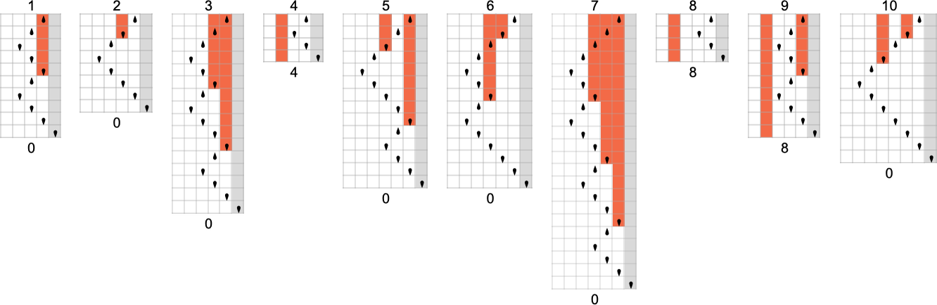
In this case, the function that the Turing machine computes is
or in graphical form:
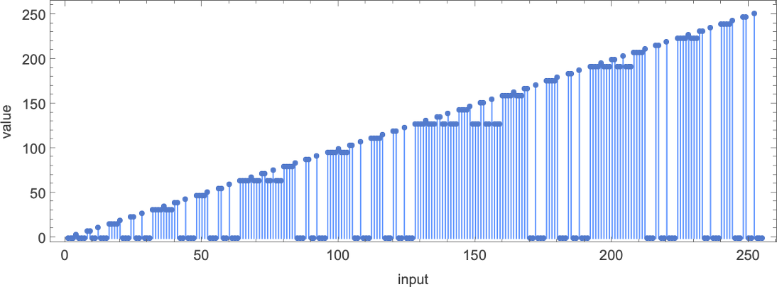
For each input, the Turing machine takes a certain number of steps to stop and give its output (i.e. the value of the function):
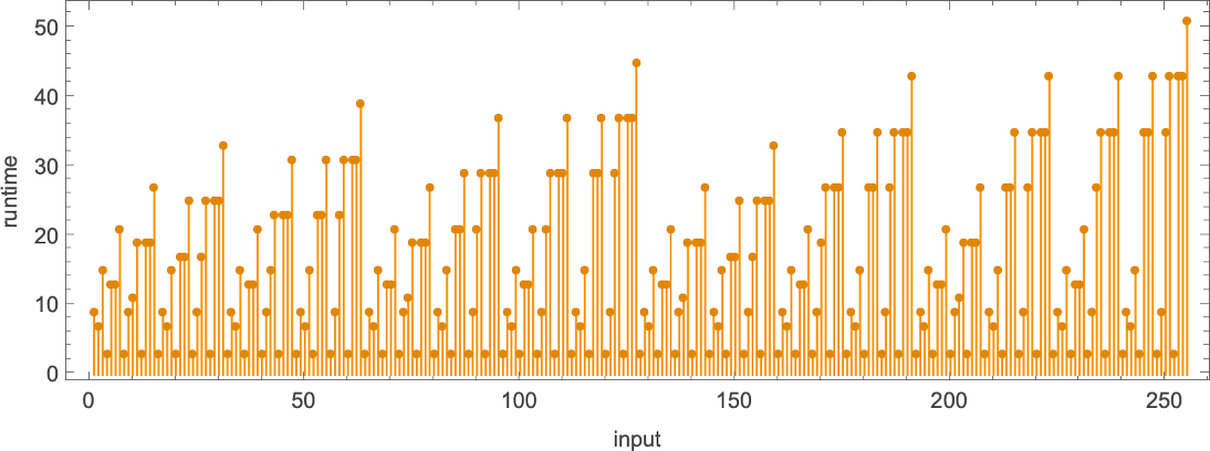
But this particular Turing machine isn’t the only one that can compute this function. Here are two more:
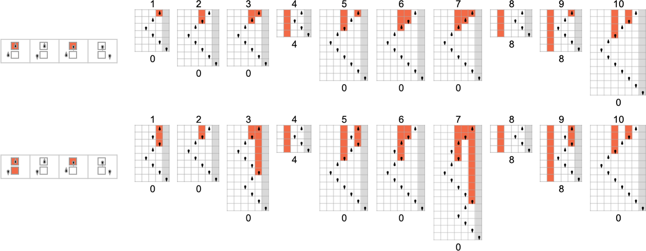
The outputs are the same as before, but the runtimes are different:
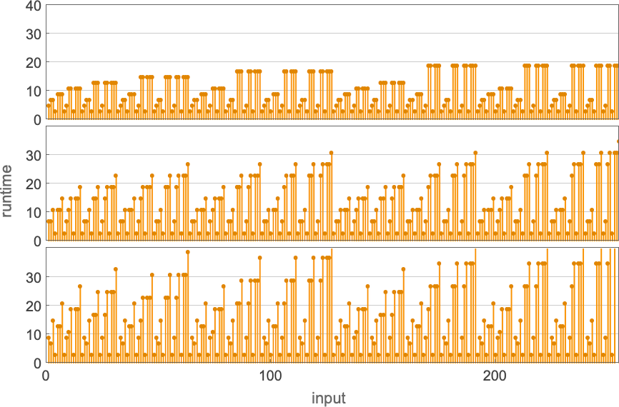
Indicating these respectively by ![]()
![]()
![]() and plotting them together, we see that there are definite trends—but no clear winner for “fastest program”:
and plotting them together, we see that there are definite trends—but no clear winner for “fastest program”:
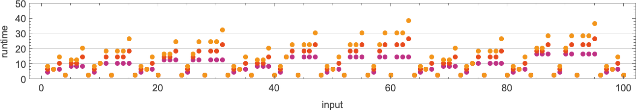
In computational complexity theory, it’s common to discuss how runtime varies with input size—which here means taking each block of inputs with a given number of digits, and just finding its maximum:
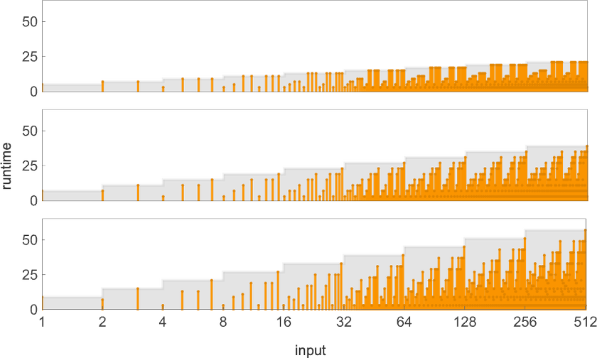
And what we see is that in this case the first Turing machine shown is “systematically faster” than the other two—and in fact provides the fastest way to compute this particular function among Turing machines of the size we’re using.
Since we’ll be dealing with lots of Turing machines here, it’s convenient to be able to specify them just with numbers—and we’ll do it the way TuringMachine in the Wolfram Language does. And with this setup, the machines we’ve just considered have numbers 261, 3333 and 1285.
In thinking about functions computed by Turing machines, there is one immediate subtlety to consider. We’ve said that we find the output by reading off what’s on the Turing machine tape when the Turing machine stops. But what if the machine never stops? (Or in our case, what if the head of the Turing machine never reaches the right-hand end?) Well, then there’s no output value defined. And in general, the functions our Turing machines compute will only be partial functions—in the sense that for some of their inputs, there may be no output value defined (as here for machine 2189):
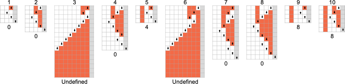
When we plot such partial functions, we’ll just have a gap where there are undefined values:
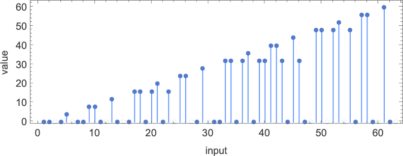
In what follows, we’ll be exploring Turing machines of different “sizes”. We’ll assume that there are two possible colors for each position on the tape—and that there are s possible states for the head. The total number of possible Turing machines with k = 2 colors and s states is (2ks)ks—which grows rapidly with s:

For any given function we’ll then be able to ask what machine (or machines) up to a given size compute it the fastest. In other words, by explicitly studying possible Turing machines, we’ll be able to establish an absolute lower bound on the computational difficulty of computing a function, at least when that computation is done by a Turing machine of at most a given size. (And, yes, the size of the Turing machine can be thought of as characterizing its “algorithmic information content”.)
In traditional computational complexity theory, it’s usually been very difficult to establish lower bounds. But our ruliological approach here will allow us to systematically do it (at least relative to machines of a given size, i.e. with given algorithmic information content). (It’s worth pointing out that if a machine is big enough, it can include a lookup table for any number of cases of any given function—making questions about the difficulty of computing at least those cases rather moot.)
To begin our systematic investigation of possible programs, let’s consider what is essentially the simplest possible case: Turing machines with one state and two possible colors of cells on their tape
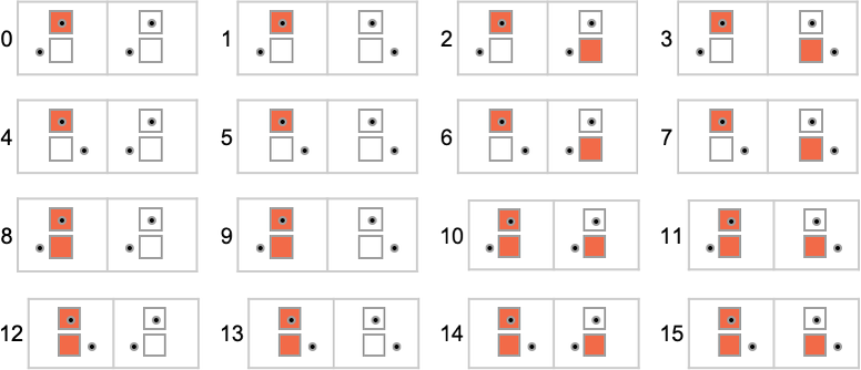
Here’s what each of these machines does for successive integer inputs:
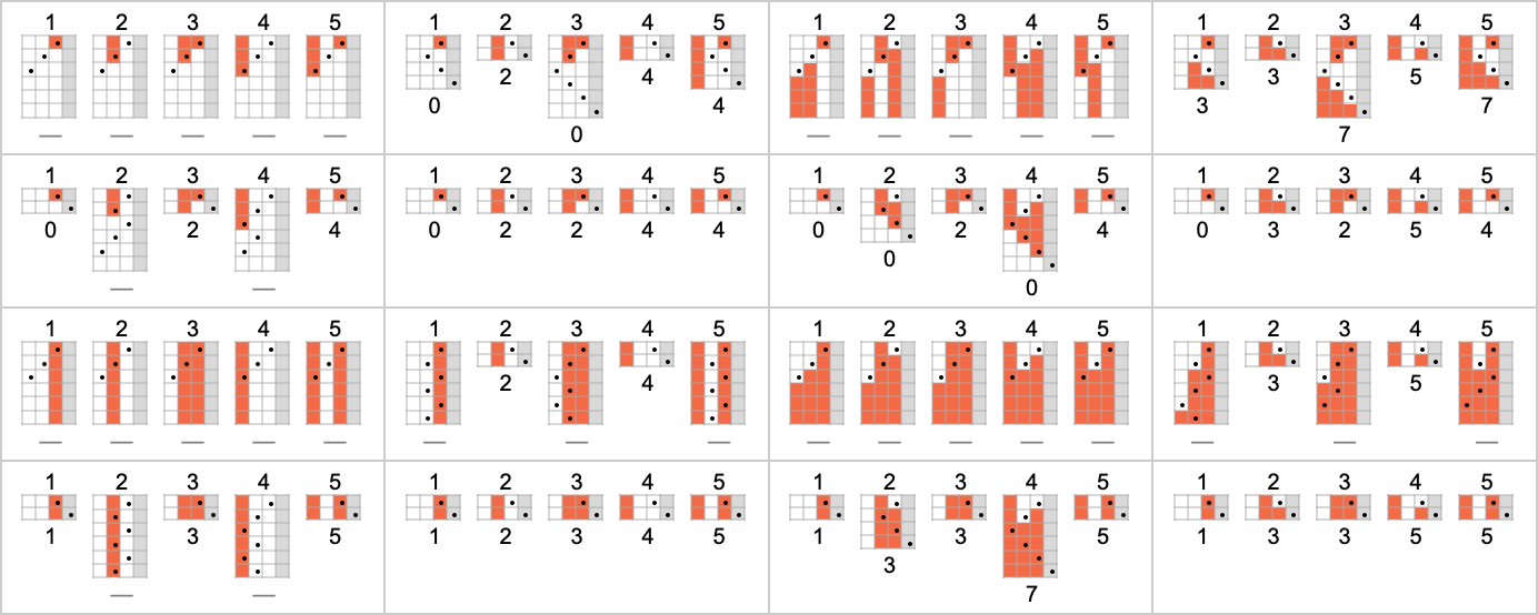
Looking at the outputs in each case, we can plot the functions these compute:
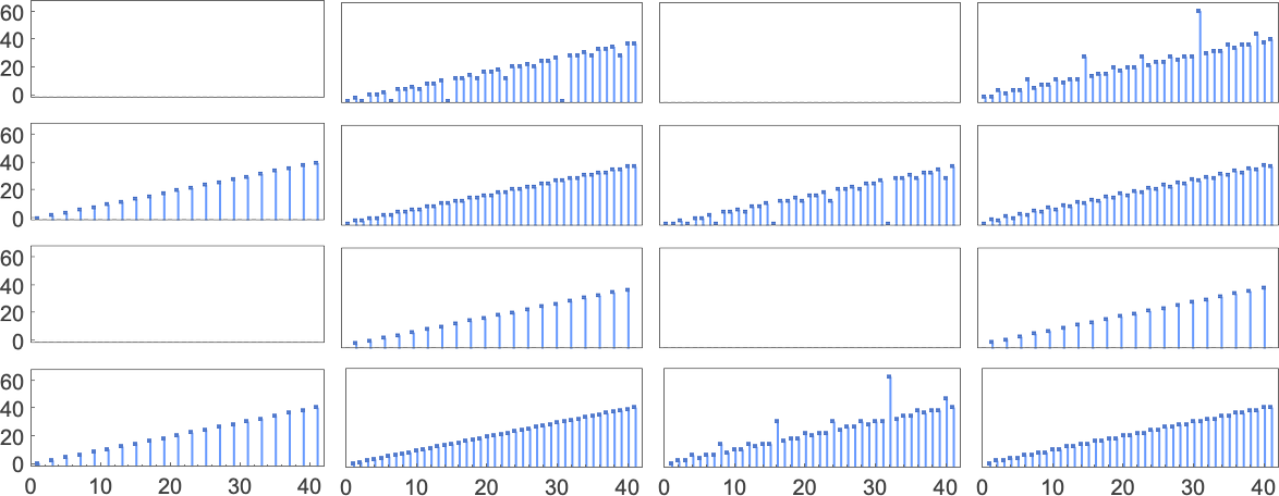
And here are the corresponding runtimes:
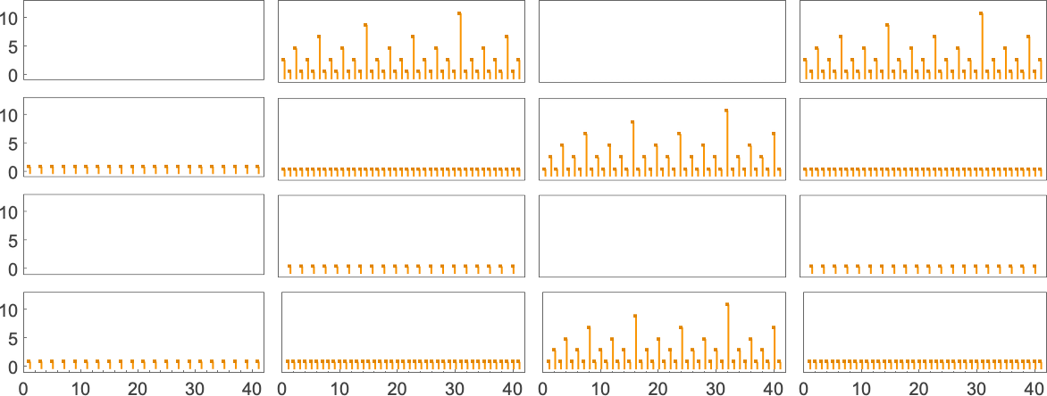
Out of all 16 machines, 8 compute total functions (i.e. the machines always terminate, so the values of the functions are defined for every input), and 8 don’t. Four machines produce “complicated-looking” functions; an example is machine 14, which computes the function:
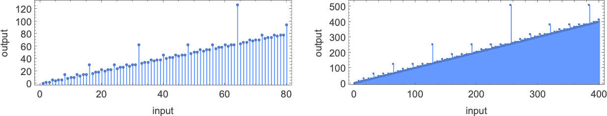
There are a variety of representations for this function, including
and:
The way the function is computed by the Turing machine is
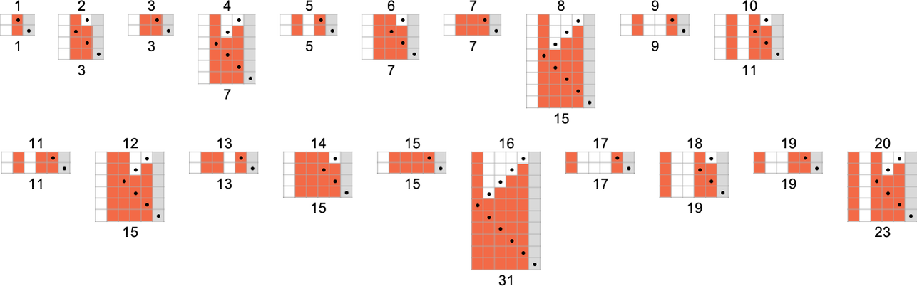
and the runtime is given by
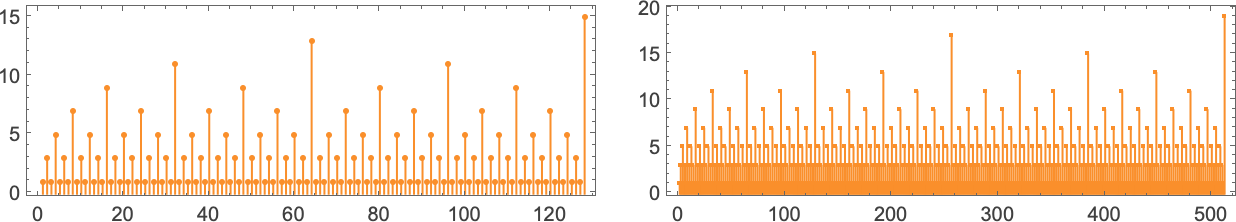
which is simply:
For input of size n, this implies the worst-case time complexity for computing this function is
Each one of the 1-state machines works at least slightly differently. But in the end, all of them are simple enough in their behavior that one can readily give a “closed-form formula” for the value of f[i] for any given i:
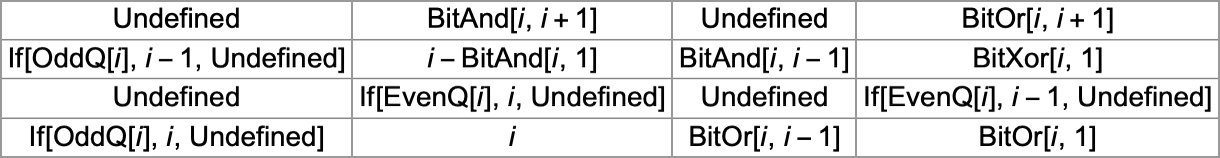
One thing that’s notable is that—except in the trivial case where all values are undefined—there are no examples among
There are a total of 4096 possible 2-state, 2-color Turing machines. Running all these machines, we find that they compute a total of 350 distinct functions—of which 189 are total. Here are plots of these distinct total functions—together with a count of how many machines generate them (altogether 2017 of the 4096 machines always terminate, and therefore compute total functions):
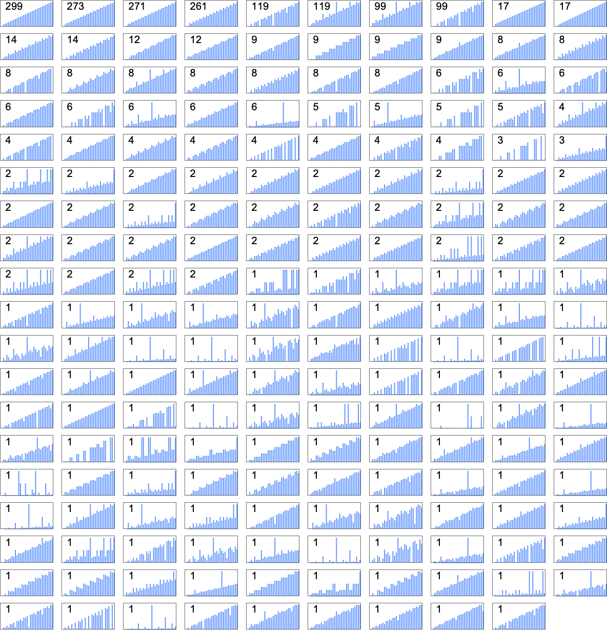
Plotting the values of all these functions in 3D, we see that the vast majority have values f[i] that are close to their inputs i—indicating that in a sense the Turing machines usually “don’t do much” to their input:
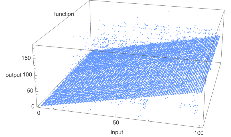
To see more clearly what the machines “actually do”, we can look at the quantity
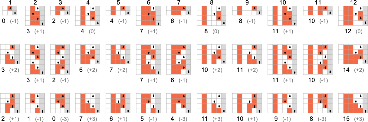
though in 6 cases it is 2, and in 3 cases (which include the “most popular” case
Dropping periodic cases, the remaining distinct

Some of what we see here is similar to the 1-state case. An example of different behavior occurs for machine 2223

which gives for
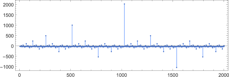
In this case f[i] turns out to be expressible simply as
or:
Another example is machine 2079
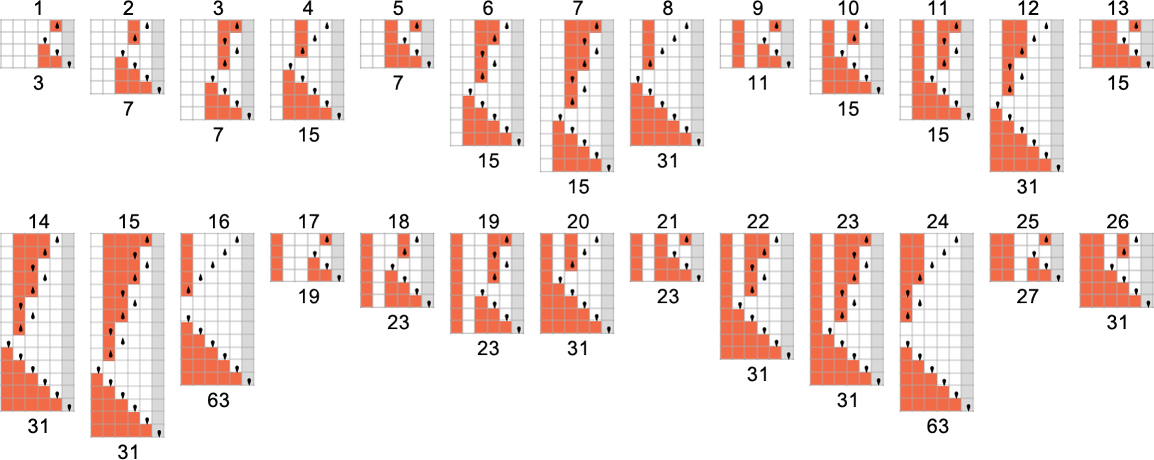
which gives for
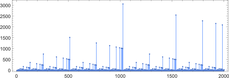
This function once again turns out to be expressible in “closed form”:
Some functions grow rapidly. For example, machine 3239
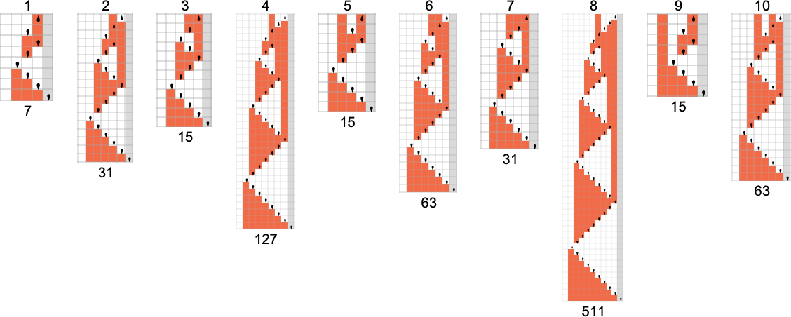
has values:
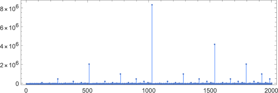
These have the property that
There are many subtleties even in dealing with 2-state Turing machines. For example, different machines may “look like” they’re generating the same function f[i] up to a certain value of i, and only then deviate. The most extreme example of such a “surprise” among machines generating total functions occurs among:
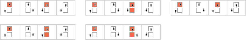
Up to
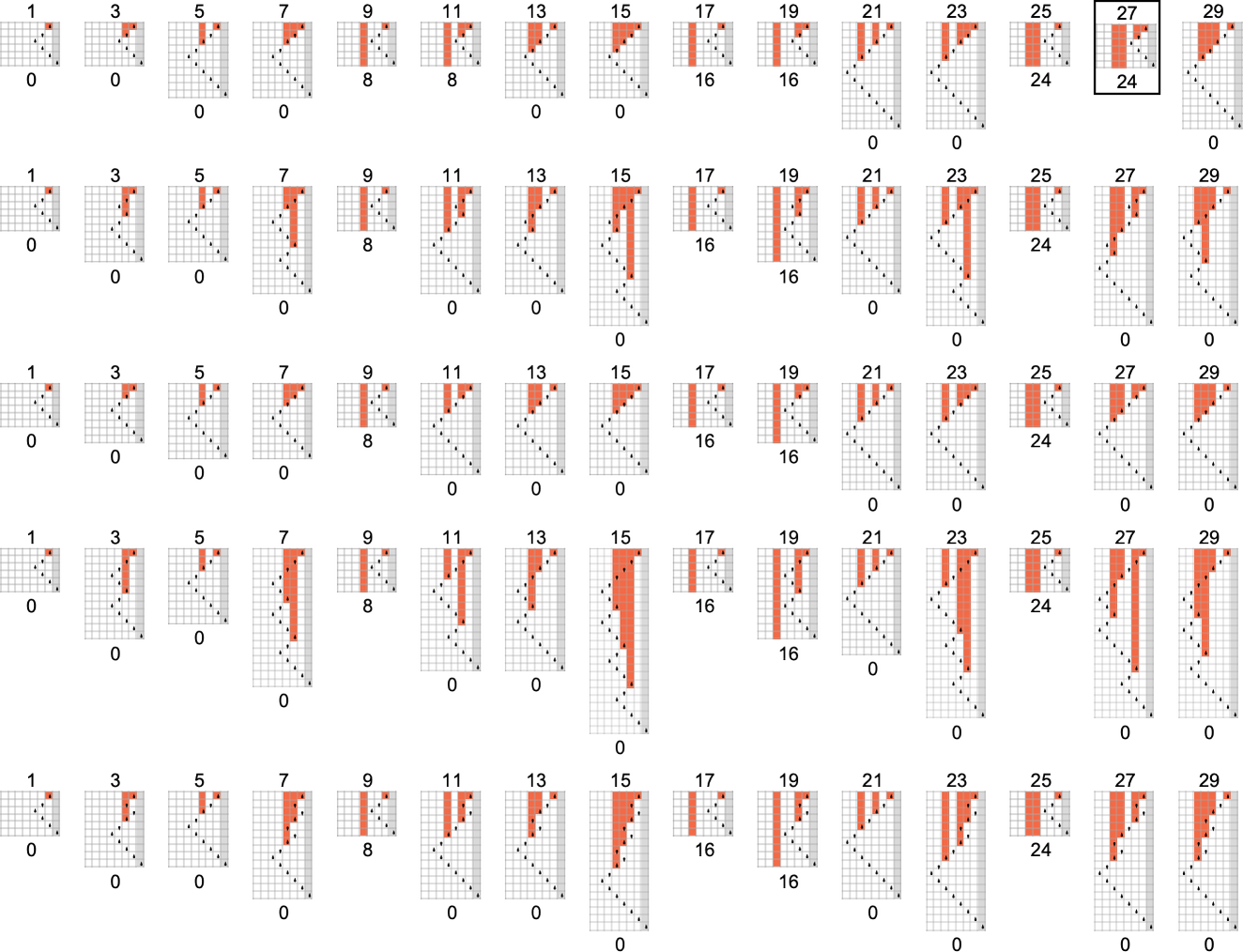
What about partial functions? At least for 2-state machines, if undefined values in f[i] are ever going to occur, they always already occur for small i. The “longest holdouts” are machines 1960 and 2972, which are both first undefined for input 8
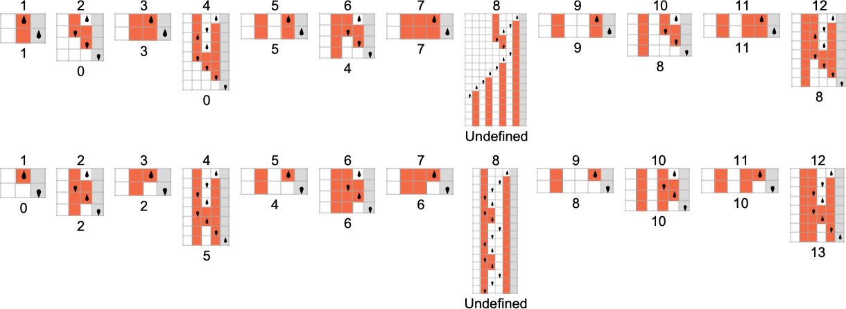
but which “become undefined” in different ways: in machine 1960, the head systematically moves to the left, while in machine 2972, it moves periodically back and forth forever, without ever reaching the right-hand end. (Despite their different mechanisms, both rules share the feature of being undefined for all inputs that are multiples of 8.)
What about runtimes? If a function f[i] is computed by several different Turing machines, the details of how it’s computed by each machine will normally be at least slightly different. Still, in many cases the mechanisms are similar enough that their runtimes are the same. And in the end, among all the 2017 machines that compute our 189 distinct total functions, there are only 103 distinct “profiles” of runtime vs. input (and indeed many of these are very similar):
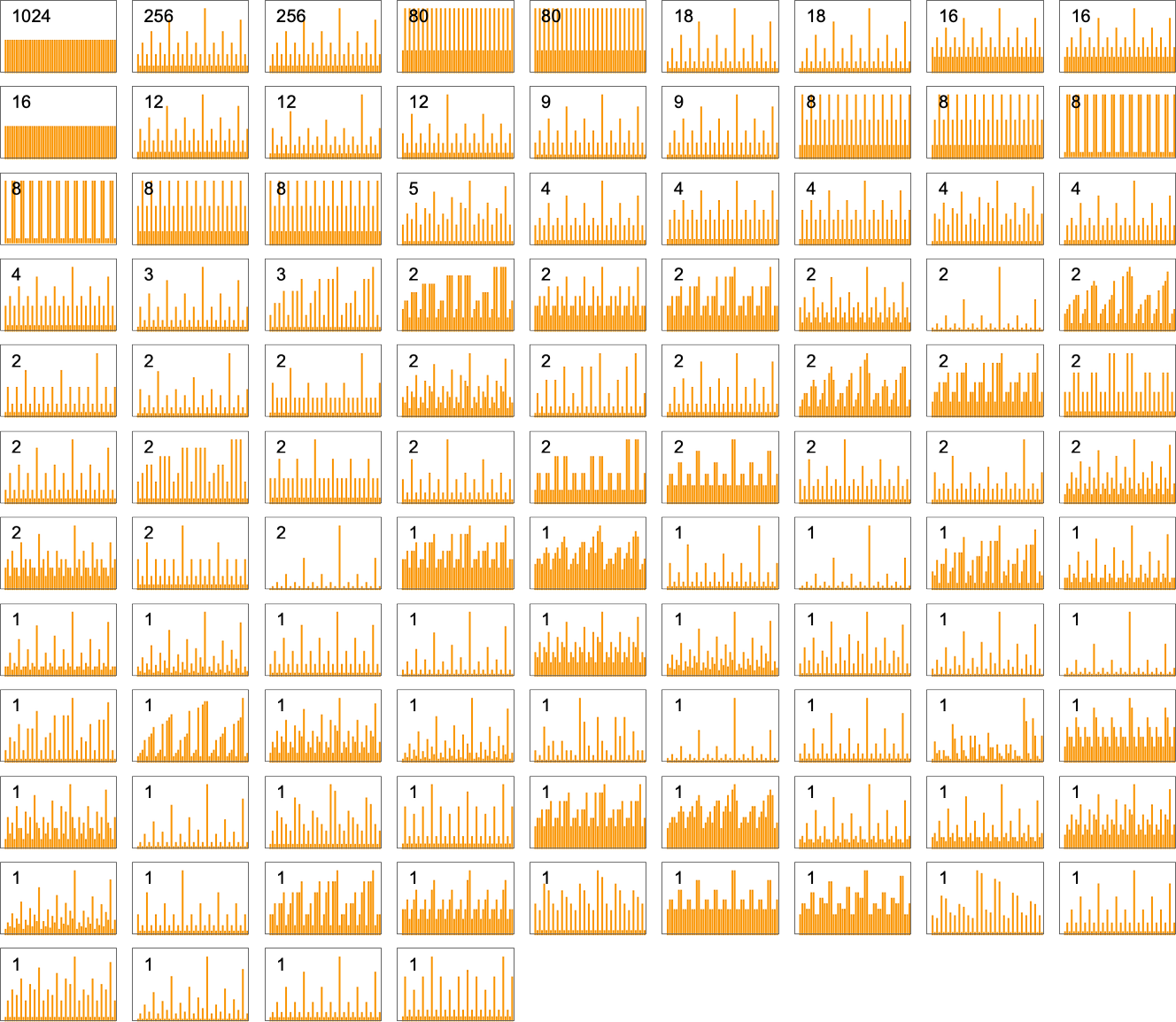
The picture gets simpler if, rather than plotting runtimes for each specific input value, we instead plot the worst-case runtime for all inputs of a given size. (In effect we’re plotting against IntegerLength[i, 2] or Ceiling[Log2[i + 1]].) There turn out to be just 71 distinct profiles for such worst-case time complexity
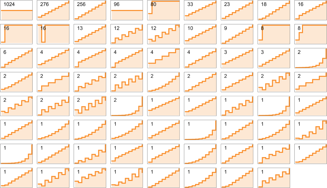
and indeed all of these have fairly simple closed forms—which for even n are (with directly analogous forms for odd n):
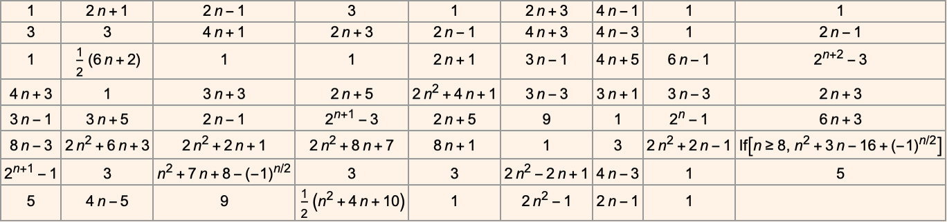
If we consider the behavior of these worst-case runtimes for large input lengths n, we find that fairly few distinct growth rates occur—notably with linear, quadratic and exponential cases, but nothing in between:
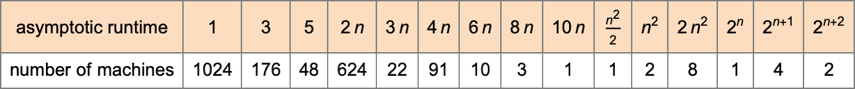
The machines with the fastest growth
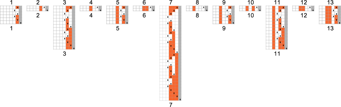
For a size-n input, the maximum value of the function is just the maximum integer with n digits, or
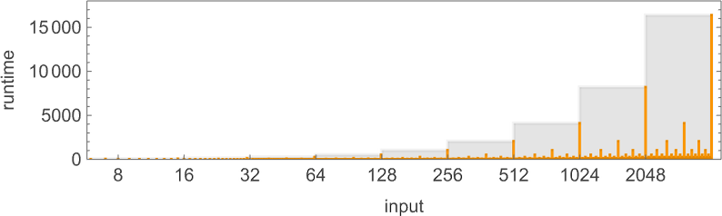
And at these maxima, the machine is effectively operating like a binary counter, generating all the states it can, with the head moving in a very regular nested pattern:
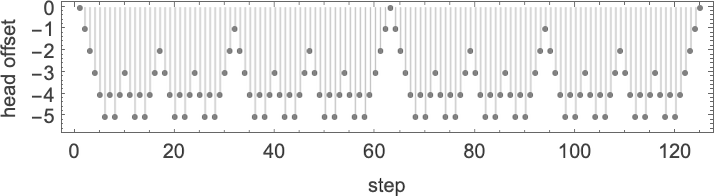
It turns out that for
Of the 8 machines with runtimes growing like
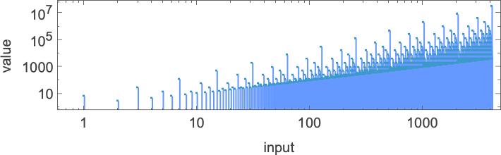
The two machines with asymptotic runtime growth
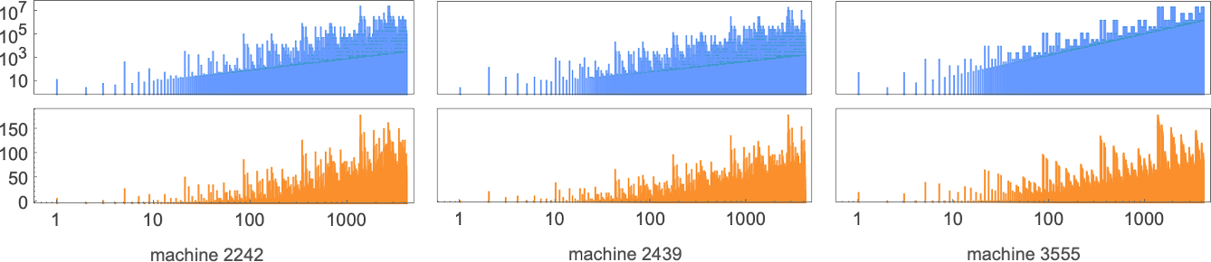
Here’s the actual behavior of these machines when given inputs 1 through 10:
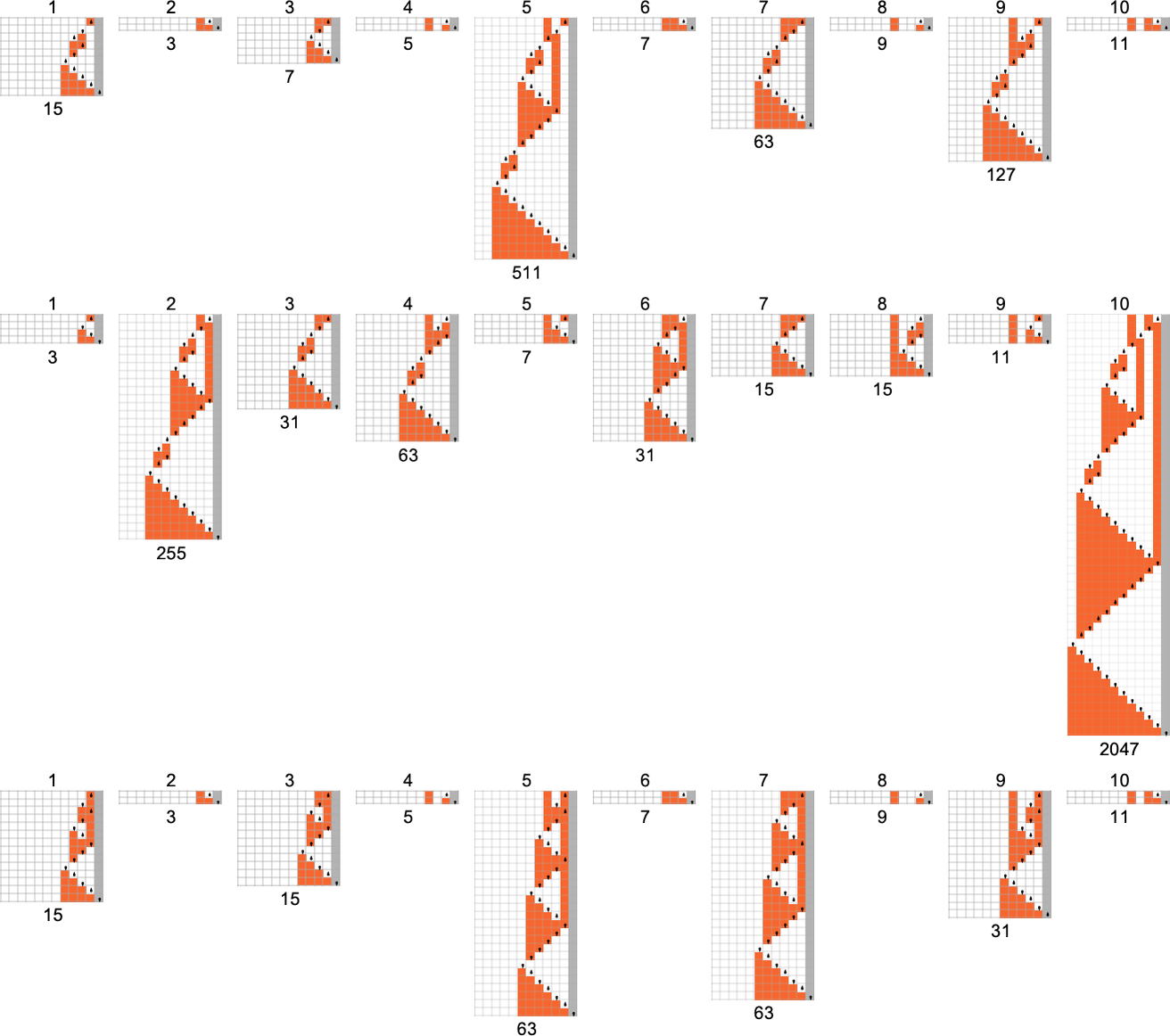
(The lack of runtimes intermediate between quadratic and exponential is notable—and perhaps reminiscent of the rarity of “intermediate growth” seen for example in the cases of finitely generated groups and multiway systems.)
Our emphasis so far has been on worst-case runtimes: the largest runtimes required for inputs of any given size. But we can also ask about the distribution of runtimes within inputs of a given size.
So, for example, here are the runtimes for all size-11 inputs for a particular, fairly typical Turing machine (
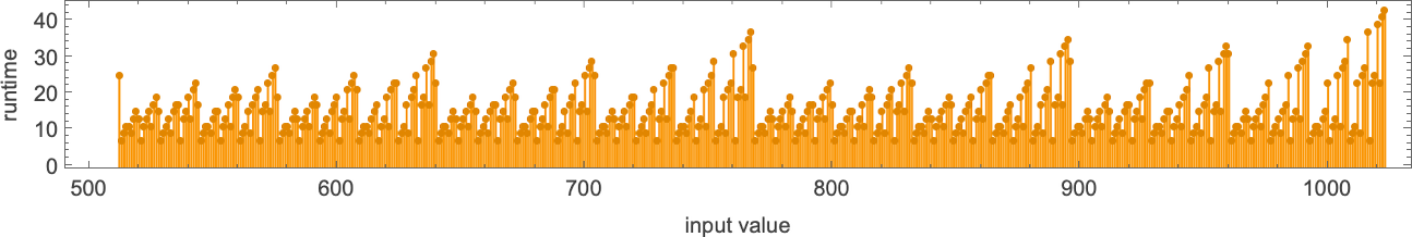
The maximum (“worst-case”) value here is 43—but the median is only 13. In other words, while some computations take a while, most run much faster—so that the runtime distribution is peaked at small values:
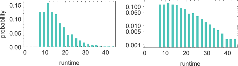
(The way our Turing machines are set up, they always run for an even number of steps before terminating—since to terminate, the head must move one position to the right for every position it moved to the left.)
If we increase the size of the inputs, we see that the distribution, at least in this case, is close to exponential:
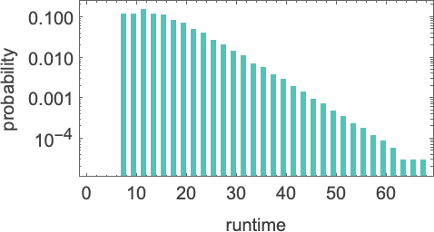
It turns out that this kind of exponential distribution is typical of what we see in almost all Turing machines. (It’s notable that this is rather different from the t –1/2 “stopping time” distribution we’d expect if the Turing machine head was “on average” executing a random walk with an absorbing boundary.) There are nevertheless machines whose distributions deviate significantly from exponential, examples being:
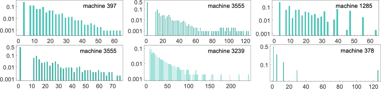
Some simply have long tails to their exponentials. Others, however, have an overall non-exponential form.
We’ve now seen lots of functions—and runtime profiles—that
We’ve seen that there are machines that compute functions quite slowly—like in exponential time. But are these machines the fastest that compute those particular functions? It turns out the answer is no.
And if we look across all 189 total functions computed by
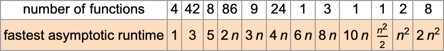
In other words, there are 8 functions that are the “most difficult to compute” for
What are these functions? Here’s one of them (computed by machine 1511):
If we plot this function, it seems to have a nested form
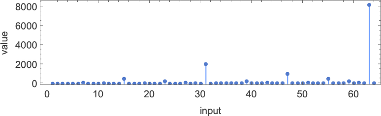
which becomes somewhat more obvious on a log-log plot:
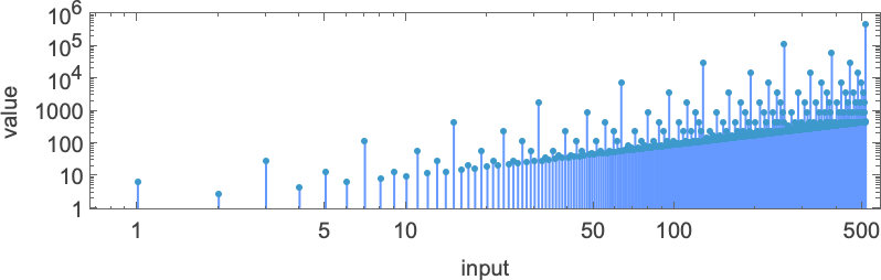
As it turns out, there’s what amounts to a “closed form” for this function
though unlike the closed forms we saw above, this one involves Nest, and effectively computes its results recursively:
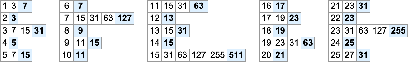
How about machine 1511? Well, here’s how it computes this function—in effect visibly using recursion:
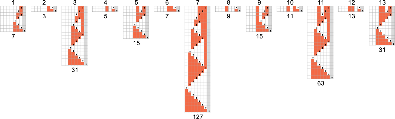
The runtimes are
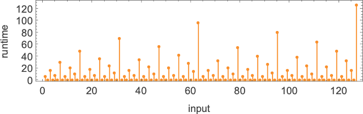
giving worst-case runtimes for inputs of size n of the form:
It turns out all 8 functions with minimum runtimes growing like
For the functions with fastest computation times
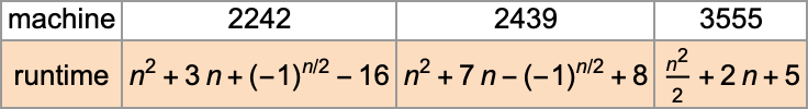
So what can we conclude? Well, we now know some functions that cannot be computed by
We now know the fastest that certain functions can be computed by
And in fact it’s common for there to be only one machine that computes a given function. Out of the 189 total functions that can be computed by
OK, but if multiple machines compute the same function, we can then ask how their speeds compare. Well, it turns out that for 145 of our 189 total functions all the different machines that compute the same function do so with the same “runtime profile” (i.e. with the same runtime for each input i). But that leaves 44 functions for which there are multiple runtime profiles:
Here are all these 44 functions, together with the distinct runtime profiles for machines that compute them:
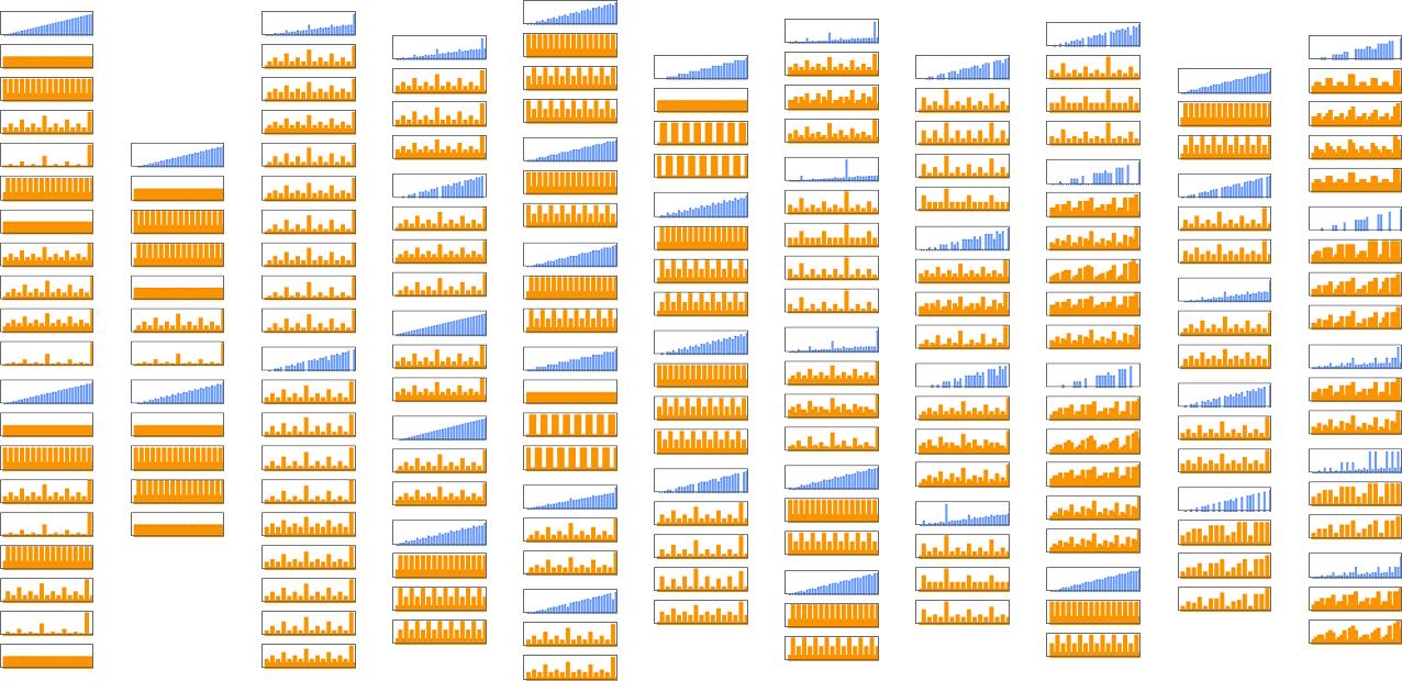
Much of the time we see that the possible runtime profiles for computing a given function differ only very little. But sometimes the difference is more significant. For example, for the identity function
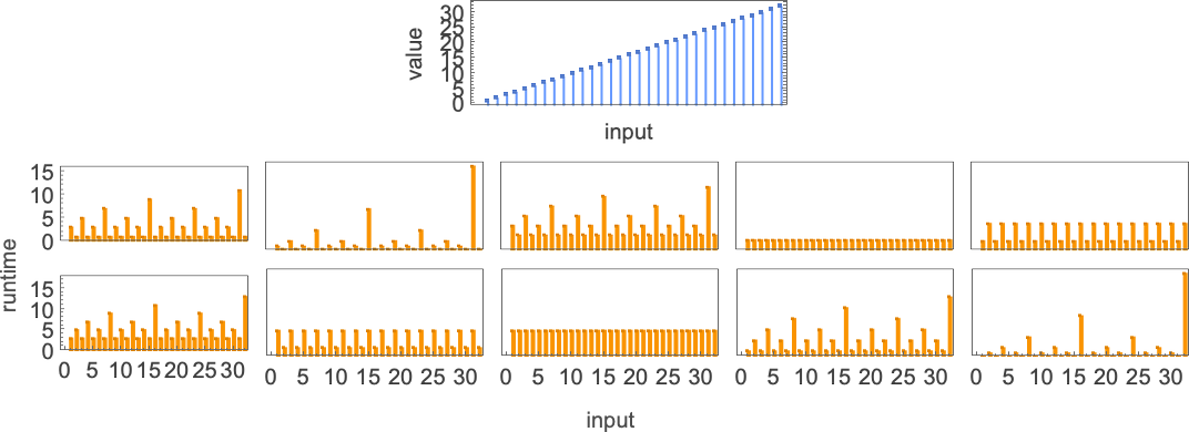
Within these 10 profiles, there are 3 distinct rates of growth for the worst-case runtime by input size: constant, linear, and exponential
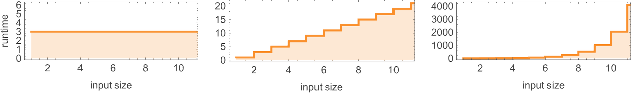
exemplified by machines 3197, 3589 and 3626 respectively:
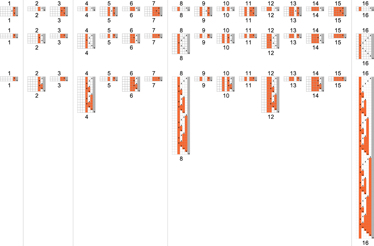
Of course, there’s a trivial way to compute this particular function—just by having a Turing machine that doesn’t change its input. And, needless to say, such a machine has runtime 1 for all inputs:
It turns out that for
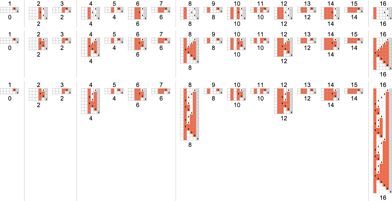
But although there are not different “orders of growth” for worst-case runtimes among any other (total) functions computed by
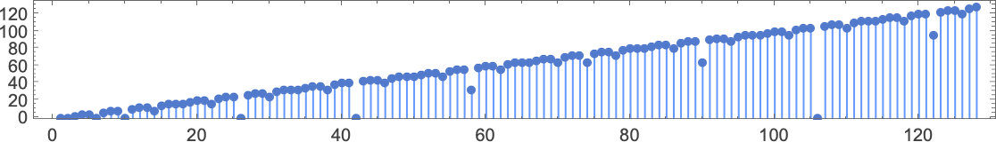
by slightly different methods
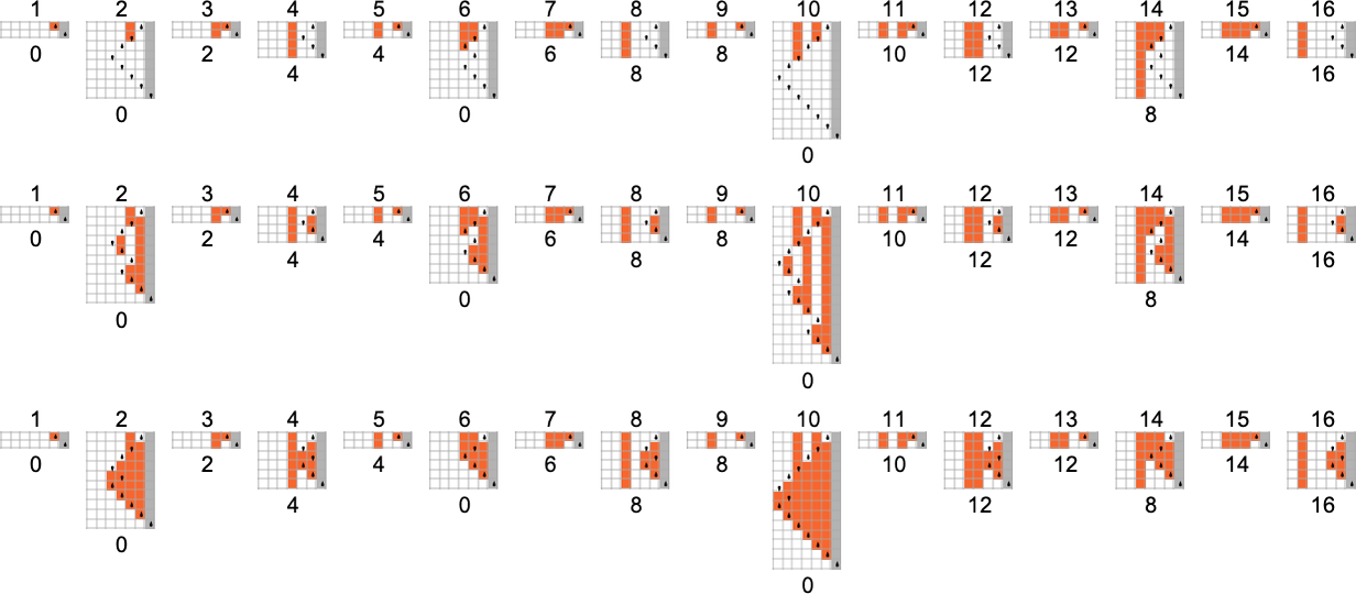
with different worst-case runtime profiles
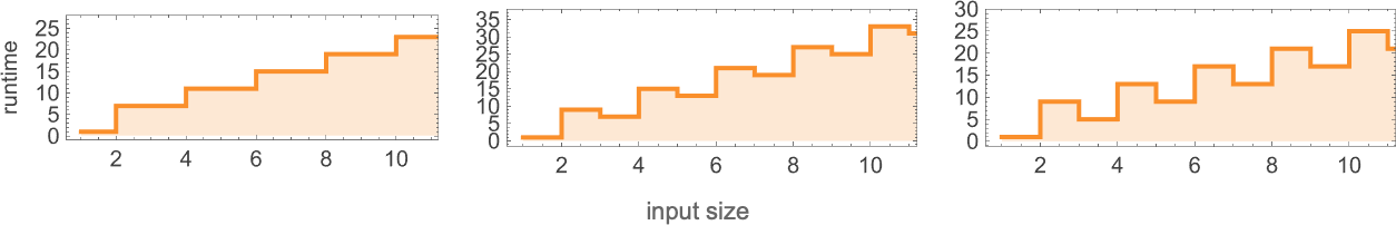
or:
By the way, if we consider partial instead of total functions, nothing particularly different happens, at least with
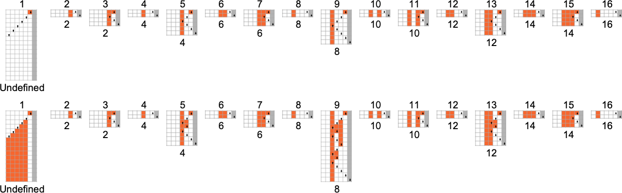
that are again essentially computing the identity function.
Another question is how
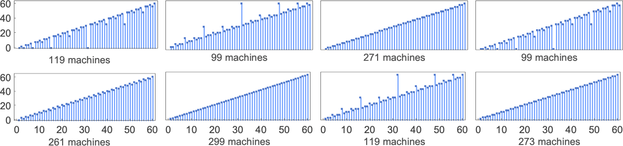
But how fast are the computations? This compares the possible worst-case runtimes for
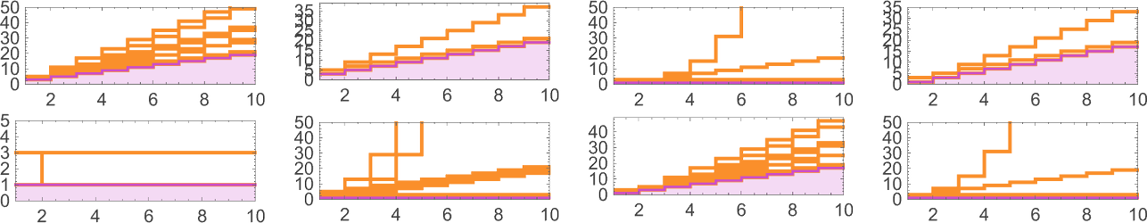
There must always be ![]() , as in:
, as in:
But can
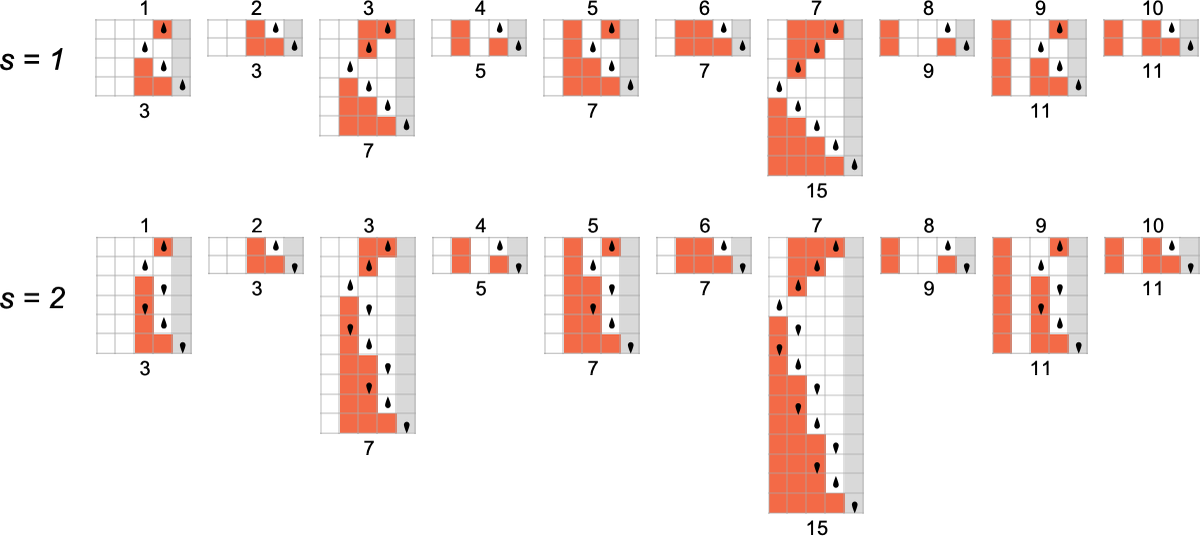
We’ve seen that different Turing machines can take different times to compute particular functions. But how fast can any conceivable Turing machine—even in principle—compute a given function?
There’s an obvious absolute lower bound to the runtime: with the way we’ve set things up, if a Turing machine is going to take input i and generate output j, its head has to at least be able to go far enough to the left to reach all the bits that need to change in going from i to j—as well as making it back to the right-hand end so that the machine halts. The number of steps required for this is
which for values of i and j up to 8 bits is:
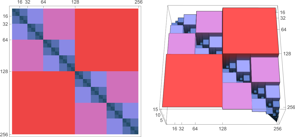
So how do the runtimes of actual Turing machine computations compare with these absolute lower bounds?
Here’s the behavior of s = 1, k = 2 machines 1 and 3, where for each input we’re giving the actual runtime along with the absolute lower bound:
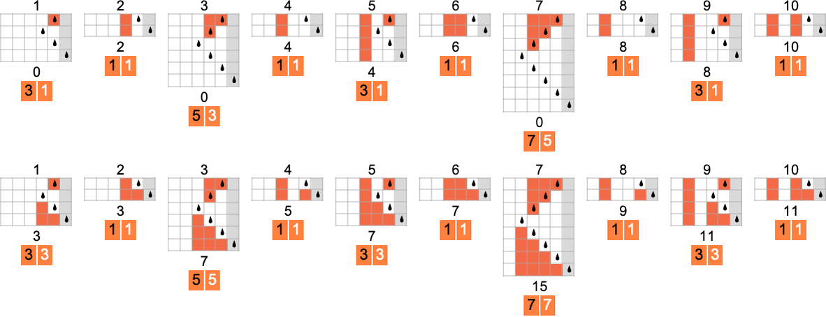
In the second case, the machine is always as efficient as it absolutely can be; in the first case, it only sometimes is—though the maximum slowdown is only 2 steps.
For s = 2, k = 2 machines, the differences can be much larger. For example, machine 378 can take exponential time—even though the absolute lower bound in this case is just 1 step, since this machine computes the identity function:
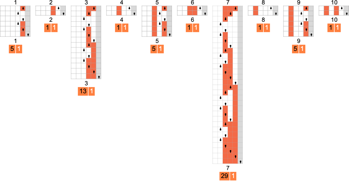
Here’s another example (machine 1447) in which the actual runtime is always roughly twice the absolute lower bound:
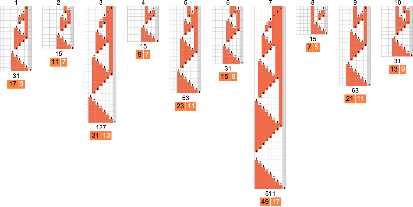
But how does the smallest (worst-case) runtime for any s = 2 Turing machine to compute a given function compare to the absolute lower bound? Well, in a result that presages what we’ll see later in discussing the P vs. NP question, the difference can be increasingly large:
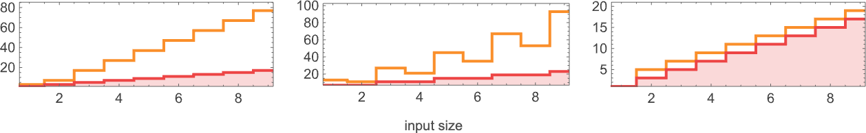
The functions being computed here are
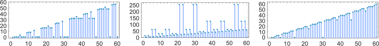
and the fastest s = 2 Turing machines that do this are (machines 2205, 3555 and 2977):
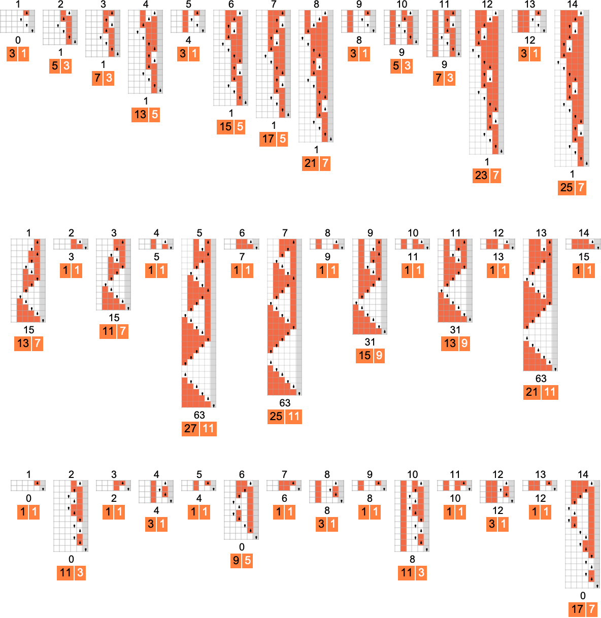
Our absolute lower bound determines how fast a Turing machine can possibly generate a given output. But one can also think of it as something that measures how much a Turing machine has “achieved” when it generates a given output. If the output is exactly the same as the input, the Turing machine has effectively “achieved nothing”. The more they differ, the more one can think of the machine having “achieved”.
So now a question one can ask is: are there functions where little is achieved in the transformation from input to output, but where the minimum runtime to perform this transformation is still long? One might wonder about the identity function—where in effect “nothing is achieved”. And indeed we’ve seen that there are Turing machines that compute this function, but only slowly. However, there are also machines that compute it quickly—so in a sense its computation doesn’t need to be slow.
The function above computed by machine 2205 is a somewhat better example. The (worst-case) “distance” between input and output grows like 2n with the input size n, but the fastest the function can be computed is what machine 2205 does, with a runtime that grows like 10n. Yes, these are still both linear in n. But at least to some extent this is an example of a function that “doesn’t need to be slow to compute”, but is at least somewhat slow to compute—at least for any
How difficult is it to compute the value of a function, say with a Turing machine? One measure of that is the time it takes, or, more specifically, how many Turing machine steps it takes. But another measure is how much “space” it takes, or, more specifically, with our setup, how far to the left the Turing machine head goes—which determines how much “Turing machine memory” or “tape” has to be present.
Here’s a typical example of the comparison between “space” and “time” used in a particular Turing machine:
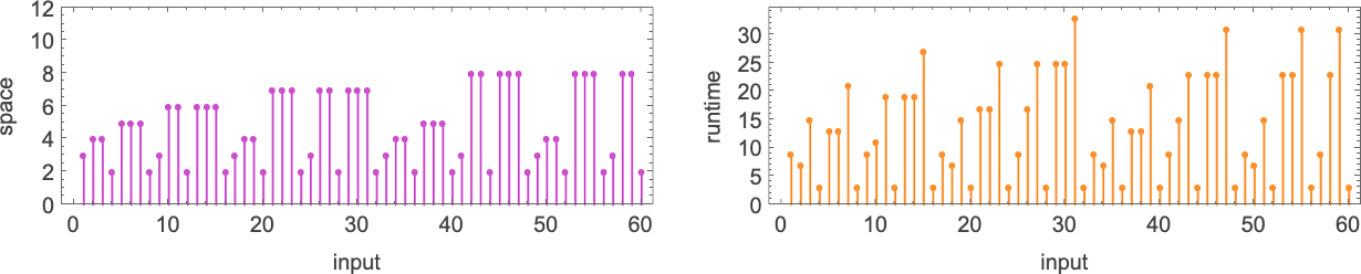
If we look at all possible space usage profiles as a function of input size we see that—at least for
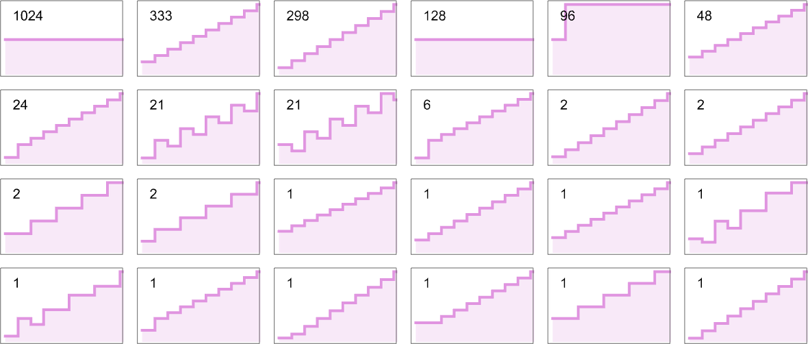
(One could also consider different measures of “complexity”—perhaps appropriate for different kinds of idealized hardware. Examples include seeing the total length of path traversed by the head, the total area of the region delimited by the head, the number of times 1 is written to the tape during the computation, etc.)
We’ve talked quite a lot about how runtime varies with input (or input size) for a particular machine. But what about the complementary question: given a particular input, how does runtime vary across different machines? Consider, for example, the
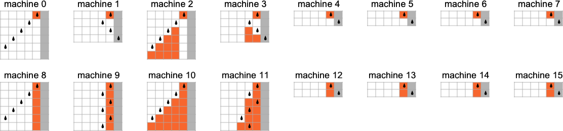
The runtimes for these machines are:
Here’s what we see if we continue to larger inputs:
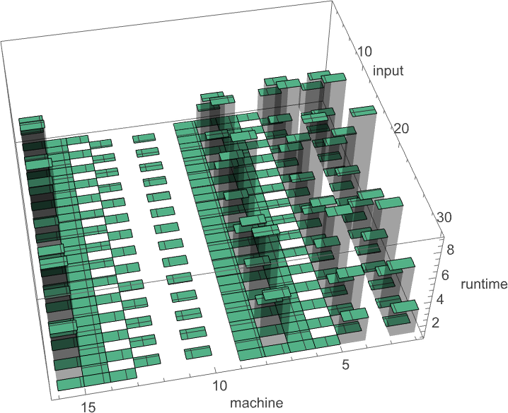
The maximum (finite) runtime across all
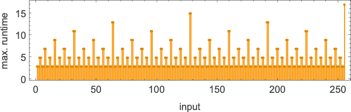
or in closed form:
For s = 2, k = 2 machines, the distribution of runtimes with input 1 is
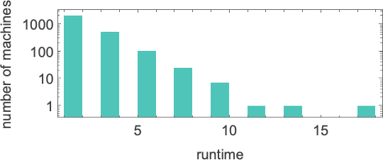
where the maximum value of 17 is achieved for machine 1447. For larger inputs the maximum runtimes are:
Plotting these maximum runtimes
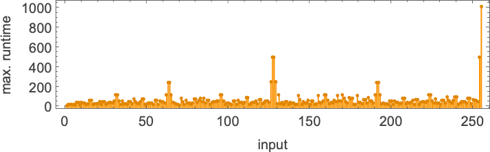
we see a big peak at input 127, corresponding to runtime 509 (achieved by machines 378 and 1351). And, yes, plotting the distribution for input 127 of runtimes for all machines, we see that this is a significant outlier:
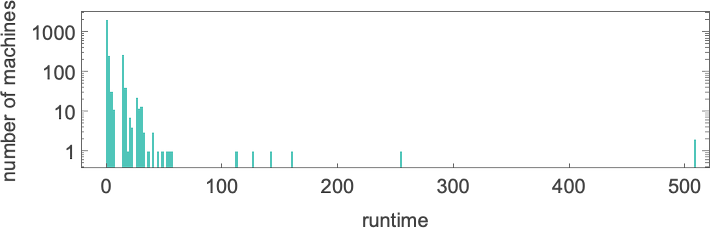
If one computes runtimes maximized over all machines and all inputs for successively larger sizes of inputs, one gets (once again dominated by machines 378 and 1351):
By the way, one can compute not only runtimes but also values and widths maximized across machines:

And, no, the maximum value isn’t always of the form
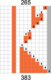
We’ve so far looked at
The issue—as so often—is of computational irreducibility. Let’s say you have a machine and you’re trying to figure out if it computes a particular function. Or you’re even just trying to figure out if for input i it gives output j. Well, you might say, why not just run the machine? And of course you can do that. But the problem is: how long should you run it for? Let’s say the machine has been running for a million steps, and still hasn’t generated any output. Will the machine eventually stop, producing either output j or some other output? Or will the machine just keep running forever, and never generate any output at all?
If the behavior of the machine was computationally reducible, then you could expect to be able to “jump ahead” and figure out what it would do, without following all the steps. But if it’s computationally irreducible, then you can’t expect to do that. It’s a classic halting problem situation. And you have to conclude that the general problem of determining whether the machine will generate, say, output j is undecidable.
Of course, in lots of particular cases (say, for lots of particular inputs) it may be easy enough to tell what’s going to happen, either just by running for some number of steps, or by using some kind of proof or other abstract derivation. But the point is that—because of computational irreducibility—there’s no upper bound on the amount of computational effort that could be needed. And so the problem of “always getting an answer” has to be considered formally undecidable.
But what happens in practice? Let’s say we look at the behavior of all
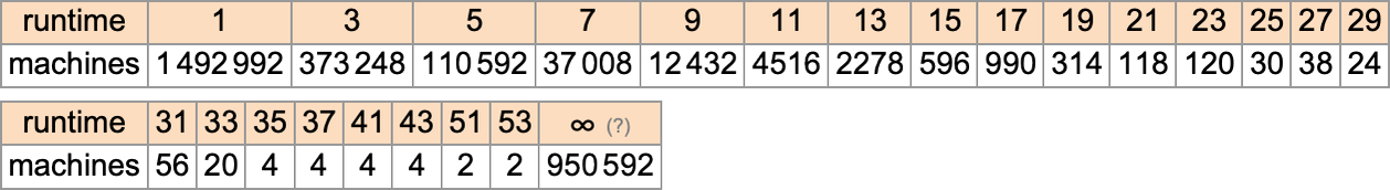
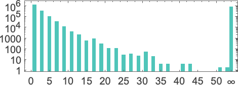
And we then conclude that a bit more than half the machines halt—with the largest finite runtime being the fairly modest 53, achieved by machine 630283 (essentially equivalent to 718804):
But is this actually correct? Or do some of the machines we think don’t halt based on running for a million steps actually eventually halt—but only after more steps?
Here are a few examples of what happens:
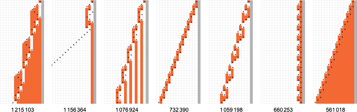
And, yes, in all these cases we can readily see that the machines will never halt—and instead, potentially after some transient, their heads just move essentially periodically forever. Here’s the distribution of periods one finds
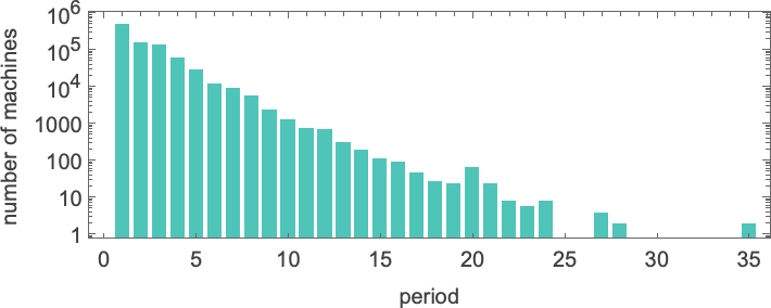
with the longest-period cases being:
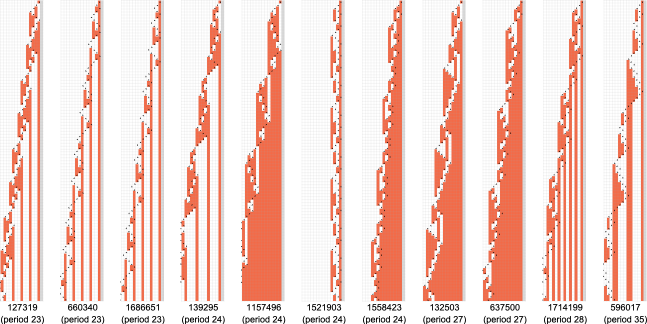
And here’s the distribution of transients
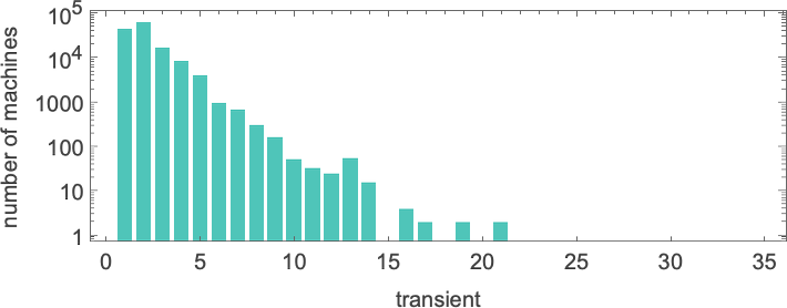
with the longest-transient cases being:
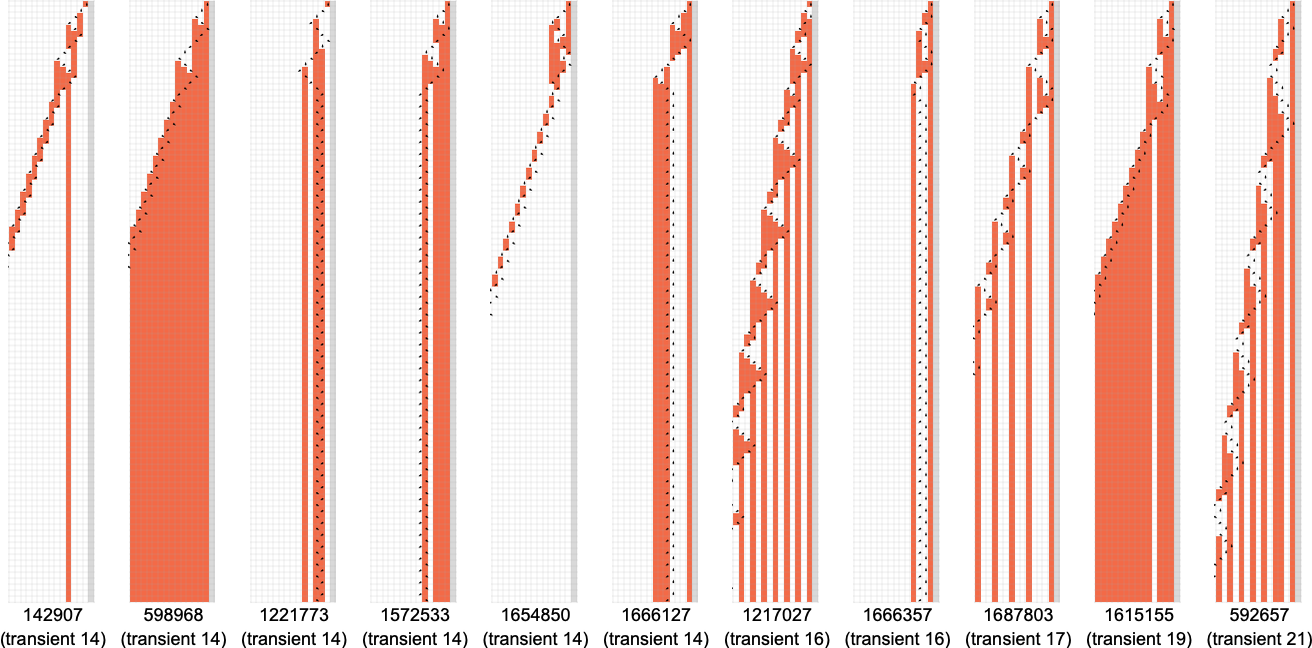
But this doesn’t quite account for all the machines that don’t halt after a million steps: there are still 1938 left over. There are 91 distinct patterns of growth—and here are samples of what happens:
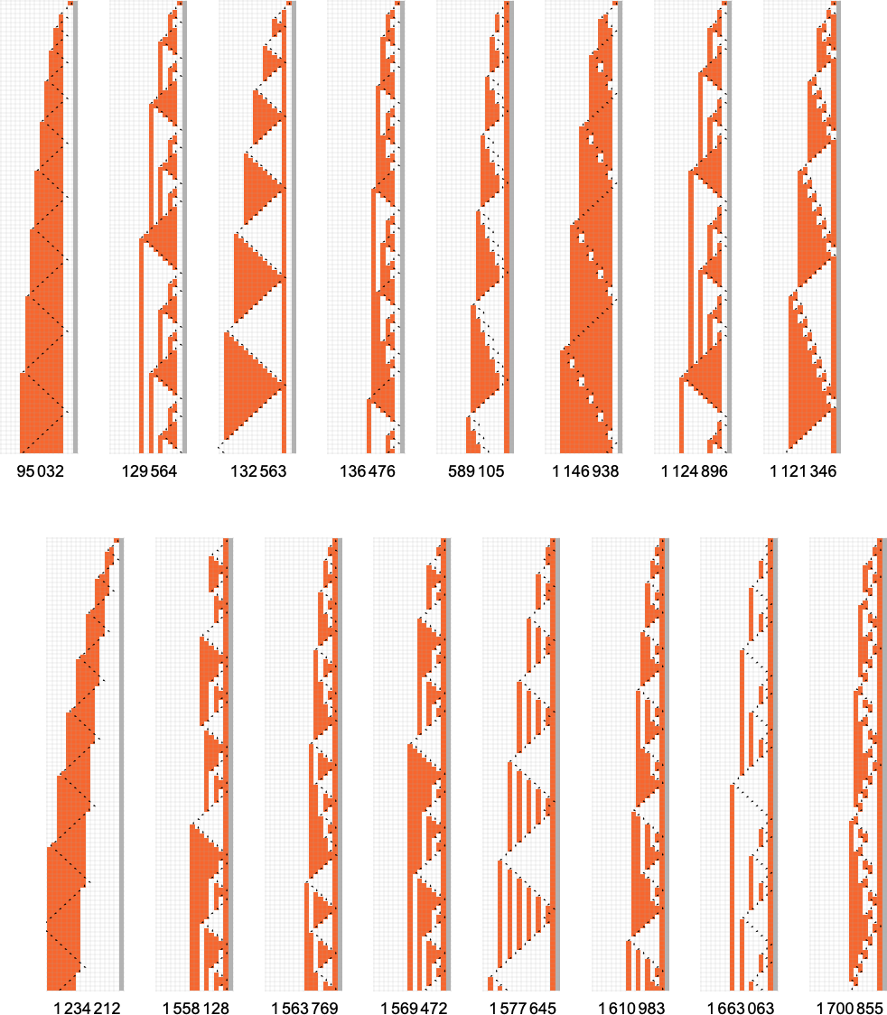
All of these eventually have a fundamentally nested structure. The patterns grow at different rates—but always in a regular succession of steps. Sometimes the spacings between these steps are polynomials, sometimes exponentials—implying either fractional power or logarithmic growth of the corresponding pattern. But the important point for our purposes here is that we can be confident that—at least with input 1—we know which
But what happens if we increase the input value we provide? Here are the first 20 maximum finite lifetimes we get:
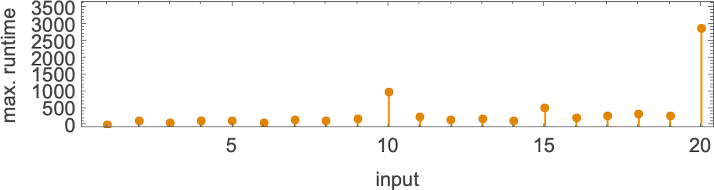
In the “peak case” of input 10, the distribution of runtimes is
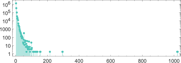
with, yes, the maximum value being a somewhat strange outlier.
What is that outlier? It’s machine 600720 (along with the related machine 670559)—and we’ll be discussing it in more depth in the next section. But suffice it to say now that 600720 shows up repeatedly as the
What about for larger inputs? Well, things get wilder then. Like, for example, consider the case of machine 1955095. For all inputs up to 41, the machine halts after a modest number of steps:
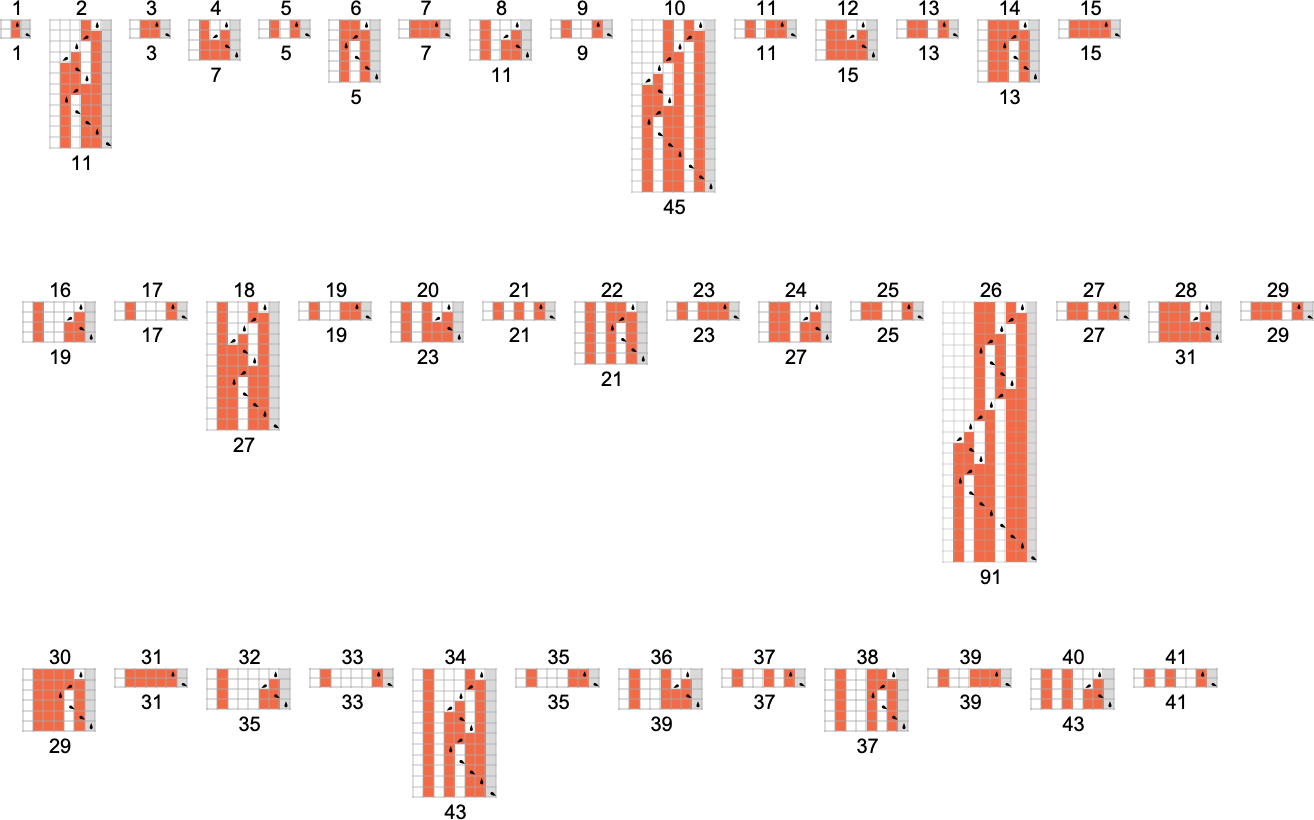
But then, at input 42, there’s suddenly a surprise—and the machine never halts:
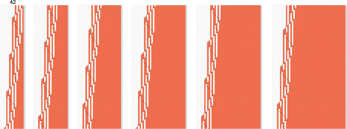
And, yes, we can immediately tell it never halts, because we can readily see that the same pattern of growth repeats periodically—every 24 steps. (A more extreme example is
And, yes, things like this are the “long arm” of undecidability reaching in. But by successively investigating both larger inputs and longer runtimes, one can develop reasonable confidence that—at least most of the time—one is correctly identifying both cases that lead to halting, and ones that do not. And from this one can estimate that of all the 2,985,984 possible
Summarizing our results we find that—somewhat surprisingly—the halting fraction is quite similar for different numbers of states, and always close to 1/2:
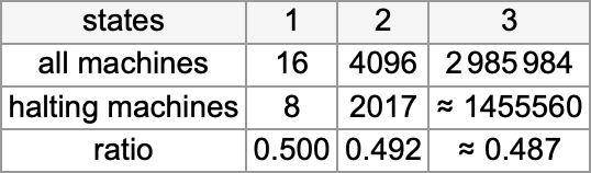
And based on our census of halting machines, we can then conclude that the number of distinct total functions computed by
In looking at the runtimes of
I actually first noticed this machine in the 1990s as part of my work on A New Kind of Science—and with considerable effort was able to give a rather elaborate analysis of at least some of its behavior:

The first remarkable thing about the machine is the dramatic peaks it exhibits in the output values it generates:
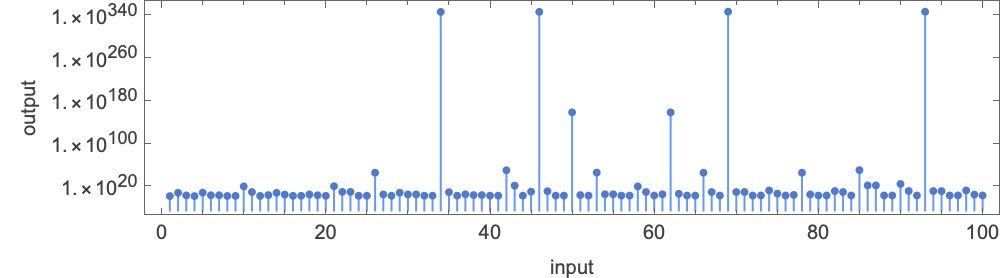
These peaks are accompanied by corresponding (somewhat less dramatic) peaks in runtime:
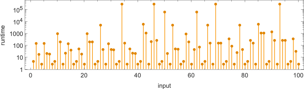
The first of the peaks shown here occurs at input i = 34—with runtime 315,391, and output
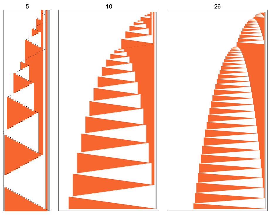
but the basic point is that the machine seems to behave in a very “deliberate” way that one might imagine could be analyzed.
It turns out, though, that the analysis is surprisingly complicated. Here’s a table of maximum (worst-case) runtimes (and corresponding inputs and outputs):
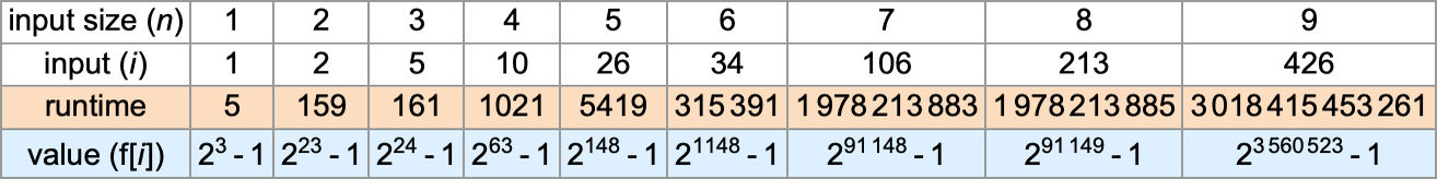
For odd n > 3, the maximum runtime occurs when the input value i is:
The corresponding initial states for the Turing machine are of the form:
The output value with such an input (for odd n > 3) is then
while the runtime—derived effectively by “mathematicizing” what the Turing machine does for these inputs—is given by the bizarrely complex formula:
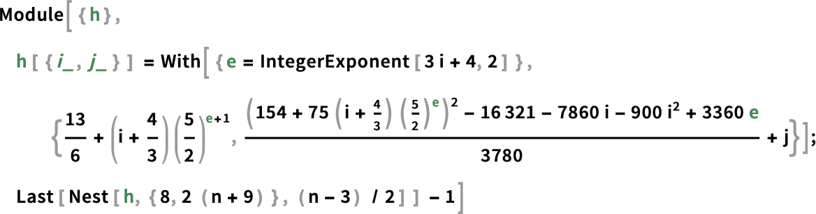
What is the asymptotic behavior? It’s roughly 6αn where α varies with n according to:
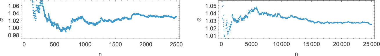
So this is how long it can take the Turing machine to compute its output. But can we find that output faster, say just by finding a “mathematical formula” for it? For inputs i with some particular forms (like the one above) it is indeed possible to find such formulas:
But in the vast majority of cases there doesn’t seem to be any simple mathematical-style formula. And indeed one can expect that this Turing machine is a typical computationally irreducible system: you can always find its output (here the value f[i]) by explicitly running the machine, but there’s no general way to shortcut this, and to systematically get to the answer by some reduced, shorter computation.
We discussed above that out of the 2.99 million possible
There are machines that give asymptotically constant runtime
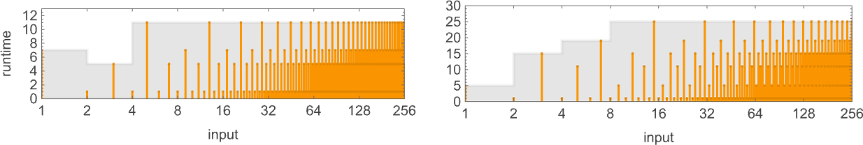
with all odd asymptotic runtime values up to 21 (along with 25) being possible:
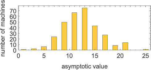
Then there are machines that give asymptotically linear runtimes, with even coefficients from 2 to 20 (along with 24)—for example:
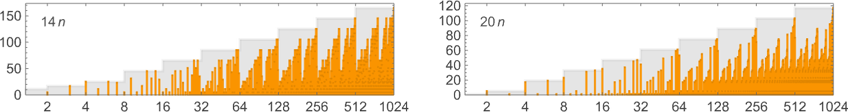
By the way, note that (as we mentioned before) some machines realize their worst-case runtimes for many specific inputs, while in other machines such runtimes are rare (here illustrated for machines with asymptotic runtimes 24n):
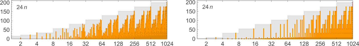
Sometimes there are machines whose worst-case runtimes increase linearly, but in effect with fractional slopes:
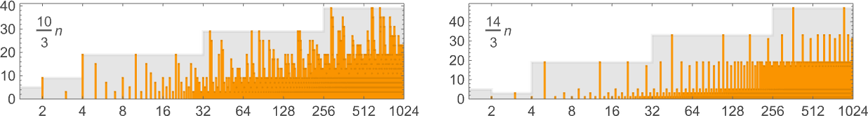
There are many machines whose worst-case runtimes increase in an ultimately linear way—but with “oscillations”:
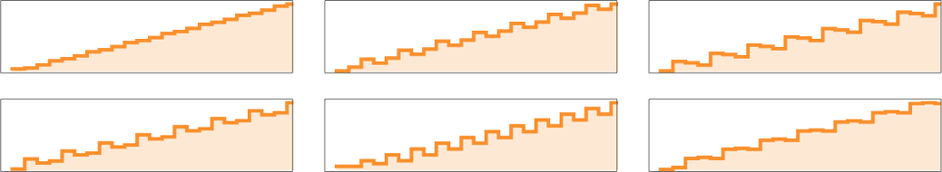
Averaging out the oscillations gives an overall growth rate of the form αn, where α is an integer or rational number with (as it turns out) denominator 2 or 3; the possible values for α are:
There are also machines with worst-case runtimes growing like αn2, with α an integer from 1 to 10 (though missing 7):
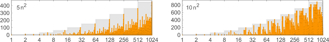
And then there are a few machines (such as 129559 and 1166261) with cubic growth rates.
The next—and, in fact, single largest—group of machines have worst-case runtimes that asymptotically grow exponentially, following linear recurrences. The possible asymptotic growth rates seem to be (ϕ is the golden ratio ![]() ):
):
Some particular examples of machines with these growth rates include (we’ll see 5n/2 and 4n examples in the next section):
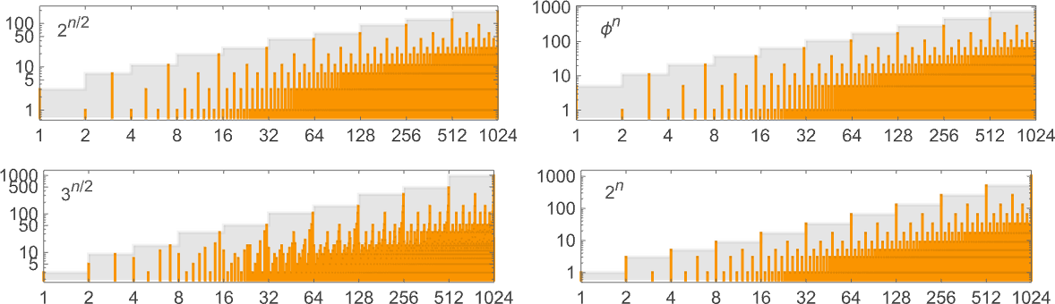
The first of these is machine 1020827, and the exact worst-case runtime for input size n in this case is:
The second case shown (machine 117245) has exact worst-case runtime
which satisfies the linear recurrence:
The third case (machine 1007039) has exact worst-case runtime:
It’s notable that in all of these cases, the maximum runtime for input size n occurs for input
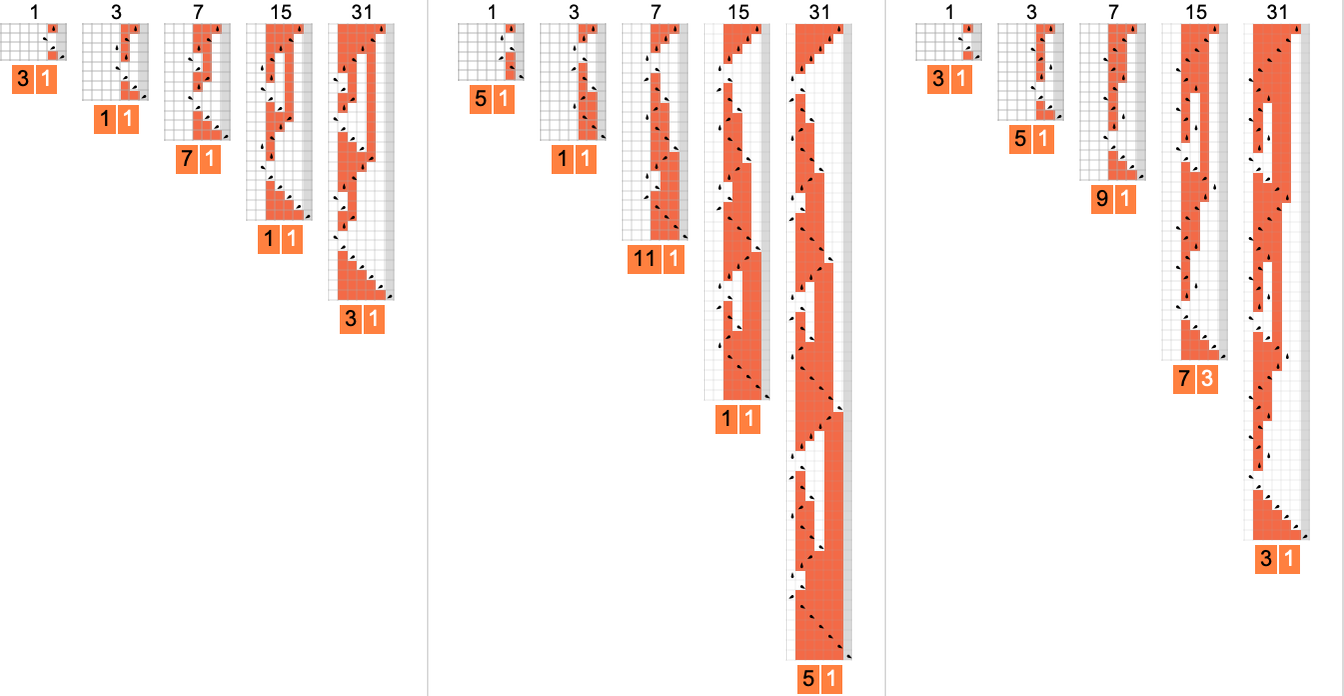
Continuing and squashing the results, it becomes clear that there’s a nested structure to these patterns:
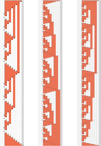
By the way, it’s certainly not necessary that the worst-case runtime must occur at the largest input of a given size. Here’s an example (machine 888388) where that’s not what happens
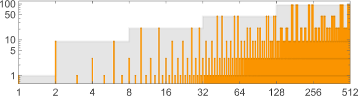
and where in the end the 2n/2 growth is achieved by having the same worst-case runtime for input sizes n and n + 1 for all even n:
One feature of everything we’ve seen here is the runtimes we’ve deduced are either asymptotically powers or asymptotically exponentials. There’s nothing in between—for example nothing like nLog[n] or 4Sqrt[n]:
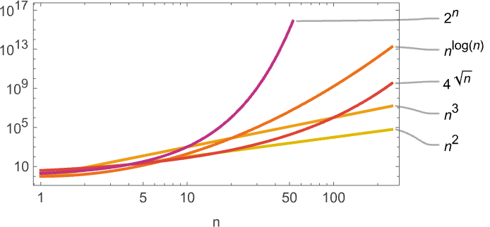
No doubt there are Turing machines with such intermediate growth, but apparently none with
As we discussed above, out of the 2.99 million possible
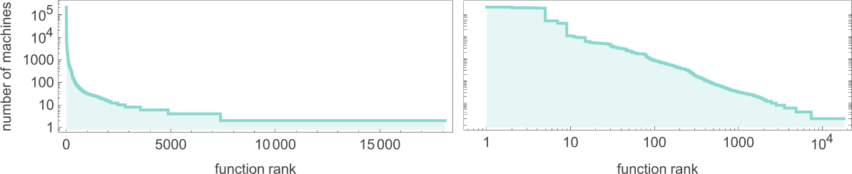
The functions computed by the most machines are (where, not surprisingly, the identity function
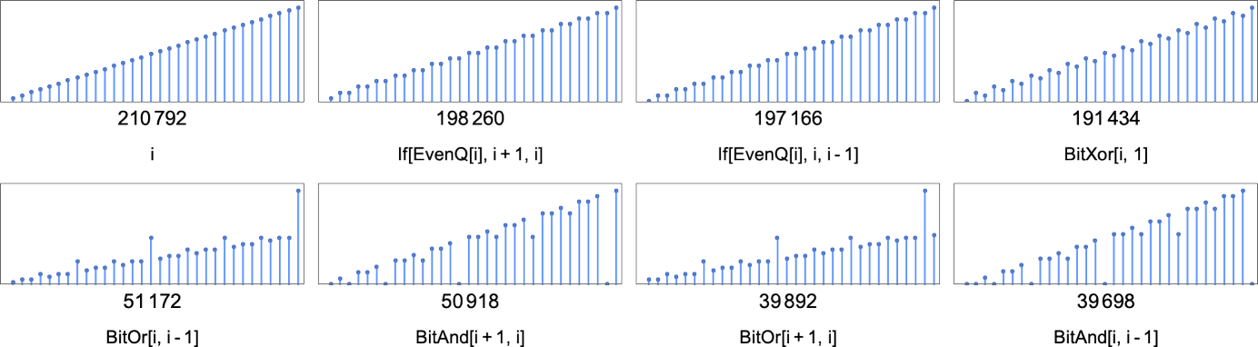
The minimum number of machines that can compute a given function is always 2—because there’s always one machine with a ![]() transition, and another with a
transition, and another with a ![]() transition, as in:
transition, as in:
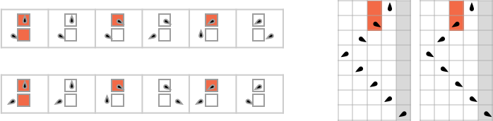
But altogether there are about 13,000 of these “isolate” machines, where no other
So what are these functions—and how long do they take to compute? And remember, these are functions that are computed by isolate machines—so whatever the runtime of those machines is, this can be thought of as defining a lower bound on the runtime to compute that function, at least by any
So what are the functions with the longest runtimes computed by isolate machines? The overall winner seems to be the function computed by machine 600720 that we discussed above.
Next appears to come machine 589111
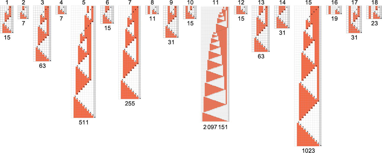
with its asymptotically 4n runtime:
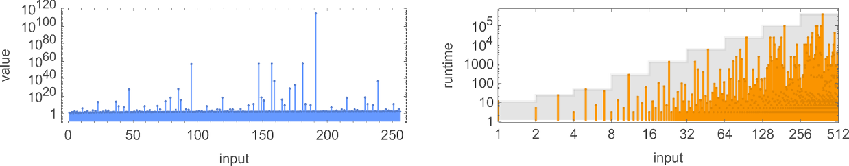
And although the values here, say for
Next appear to come machines like 599063
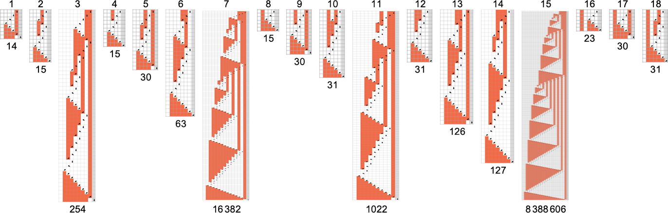
with asymptotic
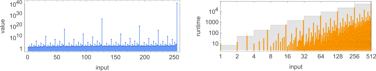
Despite the seemingly somewhat regular pattern of values for this function, the machine that computes it is an isolate, so we know that at least among
What about the other machines with asymptotically exponential runtimes that we saw in the previous section? Well, the particular machines we used as examples there aren’t even close to isolates. But there are other machines that have the same exponentially growing runtimes, and that are isolates. And, just for once, there’s a surprise.
For asymptotic runtime 2n, it turns out that there is just a single isolate machine: 1342057:
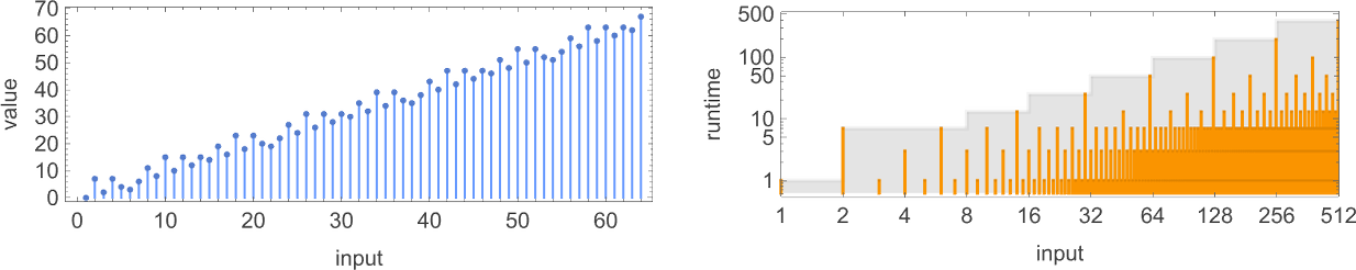
But look at how simple the function this machine computes is. In fact,
But despite the simplicity of this, it still takes the Turing machine worst-case runtime ![]() – 1
– 1
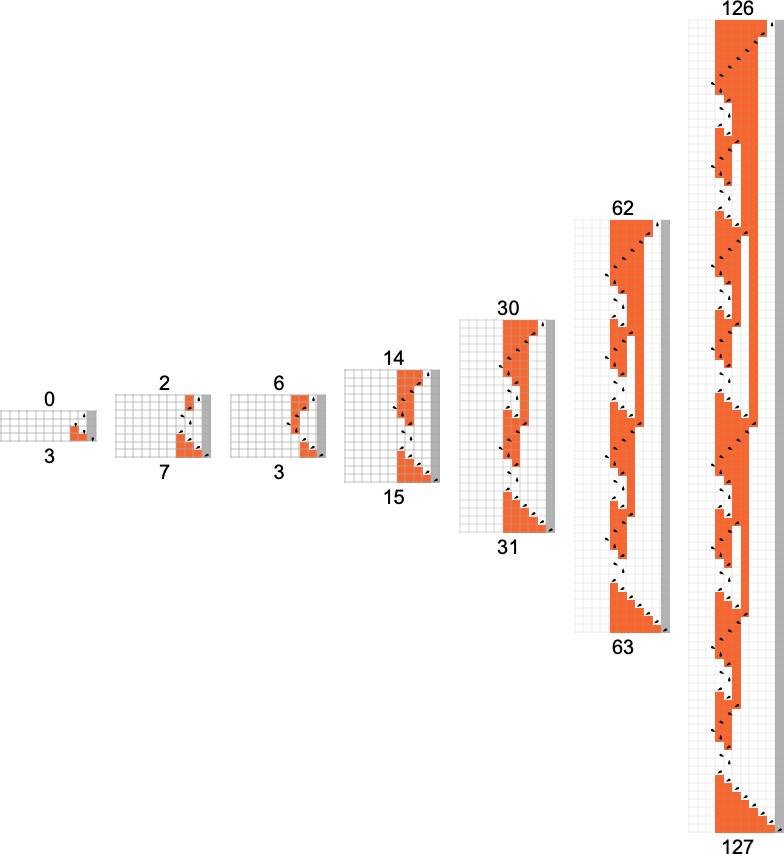
And, yes, after a transient at the beginning, all the machine is ultimately doing is to compute
Going on to asymptotic runtimes of the form 3n/2, it turns out there’s only one function for which there’s a machine (1007039) with this asymptotic runtime—and this function can be computed by over a hundred machines, many with faster runtimes, though some with slower (2n) runtimes (e.g. 879123).
What about asymptotic runtimes of order ![]() ? It’s more or less the same story as with 3n/2. There are 48 functions which can be computed by machines with this worst-case runtime. But in all cases there are also many other machines, with many other runtimes, that compute the same functions.
? It’s more or less the same story as with 3n/2. There are 48 functions which can be computed by machines with this worst-case runtime. But in all cases there are also many other machines, with many other runtimes, that compute the same functions.
But now there’s another surprise. For asymptotic runtime 2n/2 there are two functions computed only by isolate machines (889249 and 1073017):
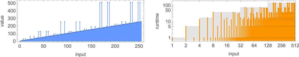
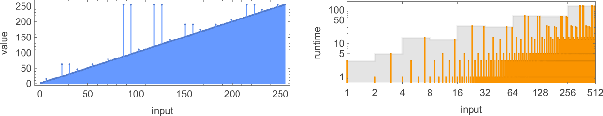
So, once again, these functions have the feature that they can’t be computed any faster by any other
When we looked at
Among
There are, of course, many more
Isolate machines immediately define lower bounds on runtime for the functions they compute. But in general (as we saw above) there can be many machines that compute a given function. For example, as mentioned above, there are 210,792
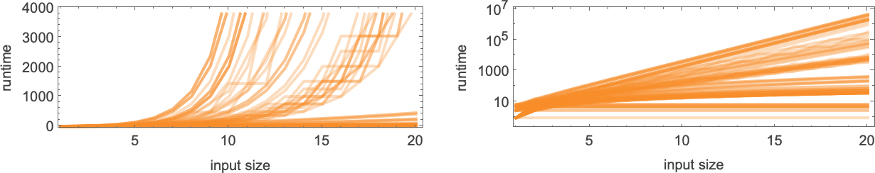
with asymptotic runtimes ranging from constant to linear, quadratic and exponential. (The most rapidly increasing runtime is ~2n.)
For each function that can be computed, there’s a slightly different collection of runtime profiles; here are the ones for the functions computed by the next largest numbers of machines:
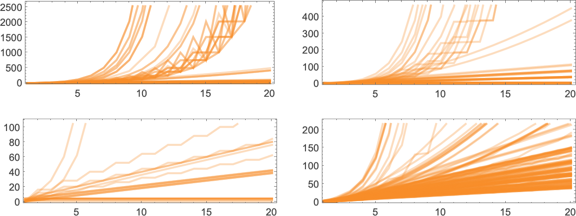
We saw above that there are functions which cannot be computed asymptotically faster than particular bounds by, say, any
The first thing to say is that (as we discussed before for
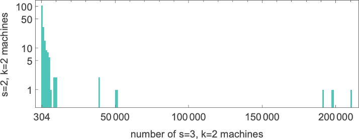
Among
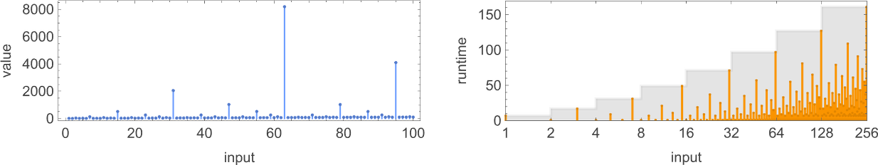
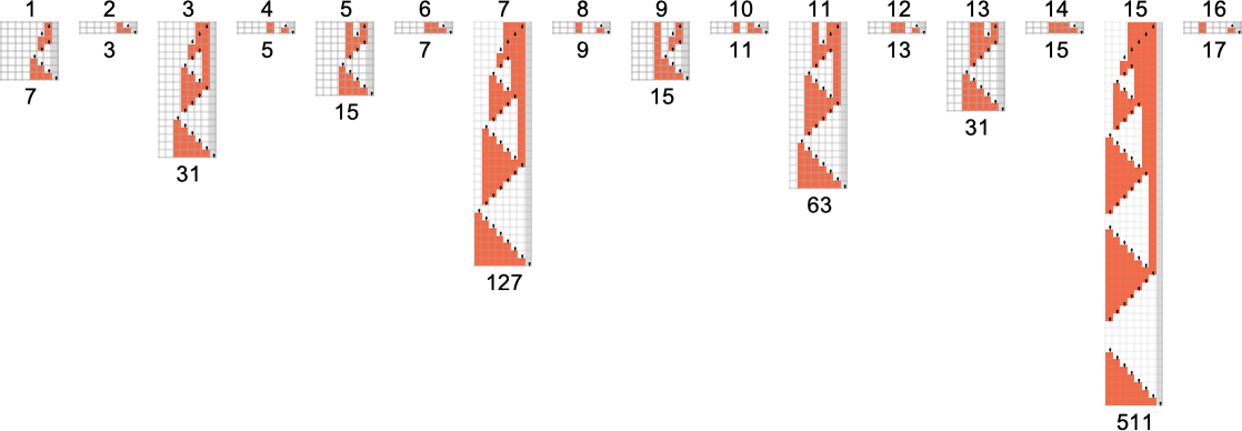
where the exact worst-case runtime is:
But now we can ask whether this function can be computed faster by any
An example is machine 1069163:
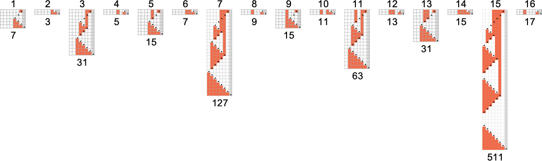
We can think of what’s happening as being that we start from the
and in effect optimize this by using a slightly more complicated “instruction set”:
In looking at
As an example, consider the function computed by the isolate machine 1342057:
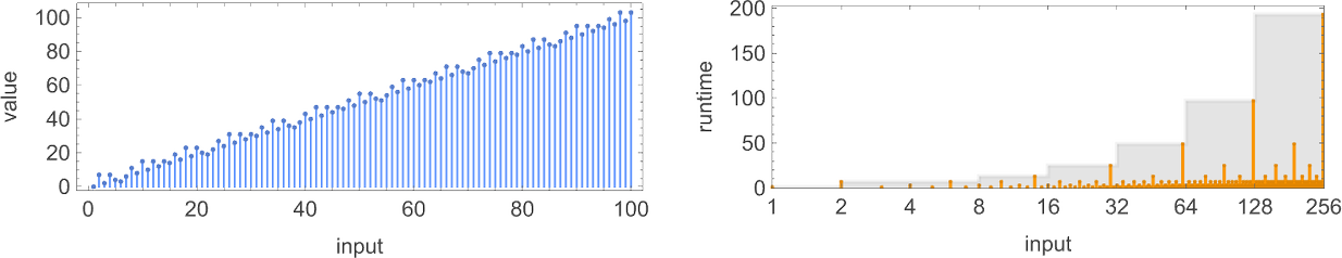
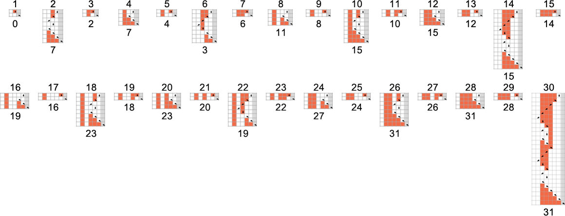
This has asymptotic runtime 4n. But now if we look at
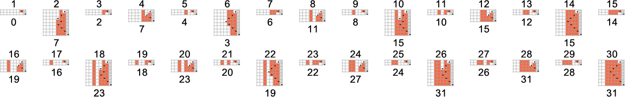
There are also machines with linearly and quadratically increasing runtimes—though, confusingly, for the first few input sizes, they seem to be increasing just as fast as our original
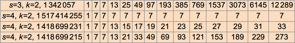
Here are the underlying rules for these particular Turing machines:
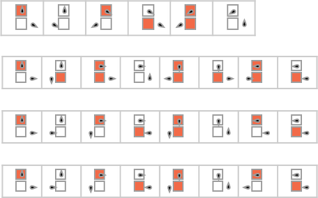
And here’s the full spectrum of runtime profiles achieved by
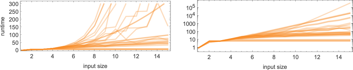
There are runtimes that are easy to recognize as exponentials—though with bases like 2,![]() , 3/2,
, 3/2, ![]() that are smaller than 4. Then there are linear and polynomial runtimes of the kind we just saw. And there’s some slightly exotic “oscillatory” behavior, like with machine 1418699063
that are smaller than 4. Then there are linear and polynomial runtimes of the kind we just saw. And there’s some slightly exotic “oscillatory” behavior, like with machine 1418699063
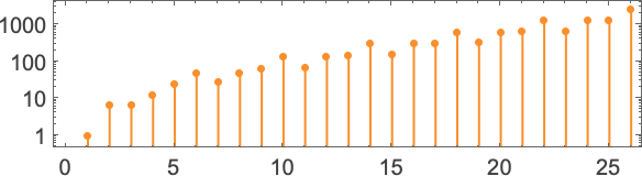
that seems to settle down to a periodic sequence of ratios, growing asymptotically like 2n/4.
What about other functions that are difficult to compute by
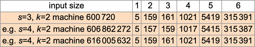
One of these follows exactly the runtimes of 600720; the other is not the same, but is very close, with about half the runtimes being the same, and the other half having maximal differences that grow linearly with n.
And what this means is that—unlike the function computed by
Looking at other functions that are “hard to compute” with
We’ve been talking so far about very small Turing machines—with at most a handful of distinct cases in their rules. But what if we consider much larger Turing machines? Would these allow us to systematically do computations much faster?
Given a particular (finite) mapping from input to output values, say
it’s quite straightforward to construct a Turing machine
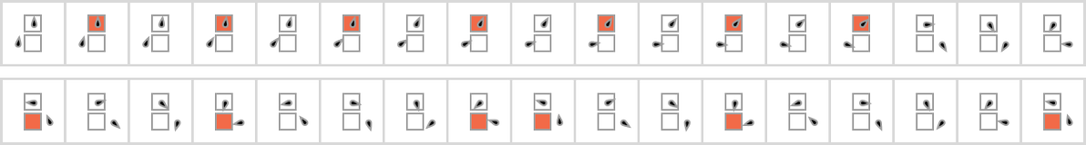
whose state transitions in effect just “immediately look up” these values:
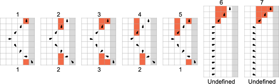
(If we try to compute a value that hasn’t been defined, the Turing machine will simply not halt.)
If we stay with a fixed value of k, then for a “function lookup table” of size v, the number of states we need for a “direct representation” of the lookup table is directly proportional to v. Meanwhile, the runtime is just equal to the absolute lower bound we discussed above, which is linearly proportional to the sizes of input and output.
Of course, with this setup, as we increase v we increase the size of the Turing machine. And we can’t guarantee to encode a function defined, say, for all integers, with anything less than an infinite Turing machine.
But by the time we’re dealing with an infinite Turing machine we don’t really need to be computing anything; we can just be looking everything up. And indeed computation theory always in effect assumes that we’re limiting the size of our machines. And as soon as we do this, there starts to be all sorts of richness in questions like which functions are computable, and what runtime is required to compute them.
In the past, we might just have assumed that there is some arbitrary bound on the size of Turing machines, or, in effect, a bound on their “algorithmic information content” or “program size”. But the point of what we’re doing here is to explore what happens not with arbitrary bounds, but with bounds that are small enough to allow us to do exhaustive empirical investigations.
In other words, we’re restricting ourselves to low algorithmic (or program) complexity and asking what then happens with time complexity, space complexity, etc. And what we find is that even in that domain, there’s remarkable richness in the behavior we’re able to see. And from the Principle of Computational Equivalence we can expect that this richness is already characteristic of what we’d see even with much larger Turing machines, and thus larger algorithmic complexity.
In everything we’ve done so far, we’ve been looking at “binary” (i.e.
The setup we’ve been using translates immediately:
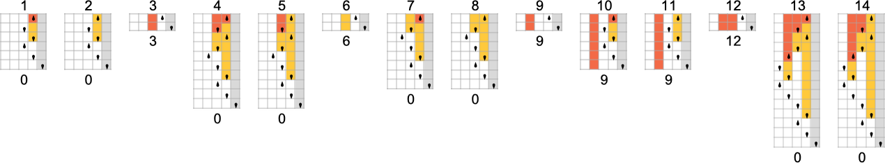
The simplest case is

Of these machines, 88 always halt—and compute 77 distinct functions. The possible runtimes are:

And unlike what we saw even for
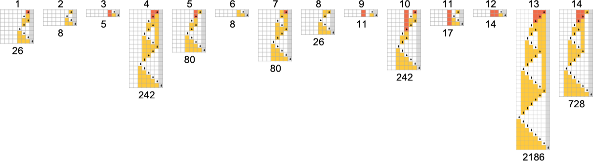
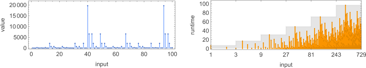
For s = 2, k = 3, we have
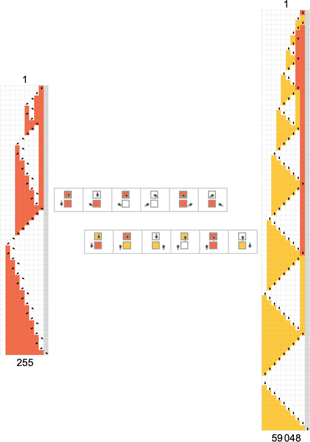
In both cases, of the machines that don’t halt, the vast majority become periodic. For
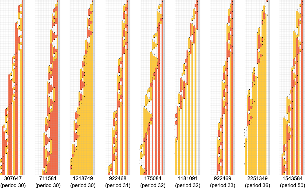
Just as for
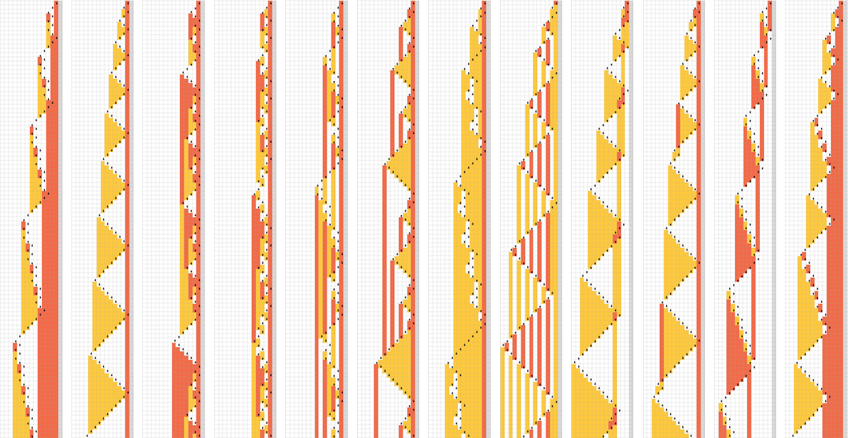
or in squashed form:
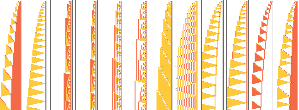
If we look beyond input 1, we find that about 1.12 million
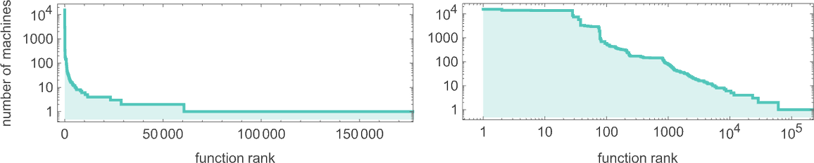
A notable feature is that the tail consists of functions computed by only one machine. In the ![]() and
and ![]() means that there are always at least two machines computing a given function. But with
means that there are always at least two machines computing a given function. But with
What about runtimes? The results for
In a sense it should not be surprising that there is so much similarity between the behavior of
However, if we look not at the kind of “one-sided” (or “halt if you go to the right”) Turing machines we are considering here, but instead at Turing machines where the head can go freely in either direction, then one difference emerges. Starting with a blank tape, all
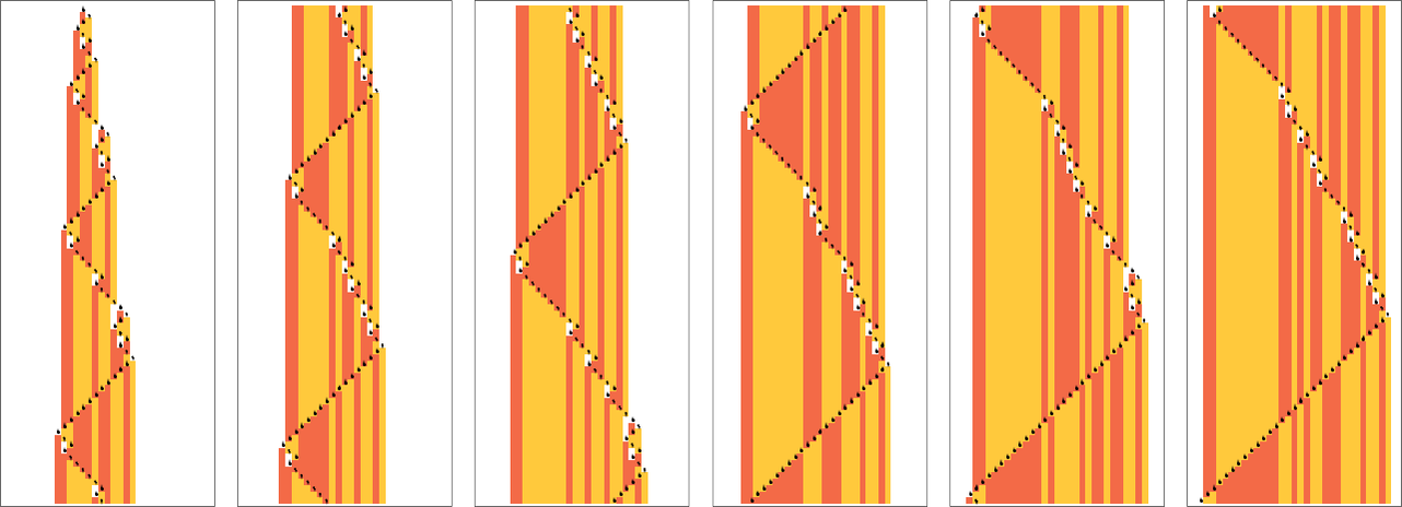
And this fact provides a clue that such a machine (or, actually, the 14 essentially equivalent machines of which this is one example) might be capable of universal computation. And indeed it can be shown that—at least with appropriate (infinite) initial conditions, the machine can successfully be “programmed” to emulate systems that are known to be universal, thereby proving that it itself is universal.
How does this machine fare with our one-sided setup? Here’s what it does with the first few inputs:
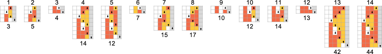
And what one finds is that for any input, the head of the machine eventually goes to the right, so with our one-sided setup we consider the machine to halt:
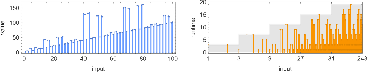
It turns out that the worst-case runtime for input of size n grows according to:
But if we look at the function computed by this machine we can ask whether there are ways to compute it faster. And it turns out there are 11 other s = 2, k = 3 machines (though, for example, no
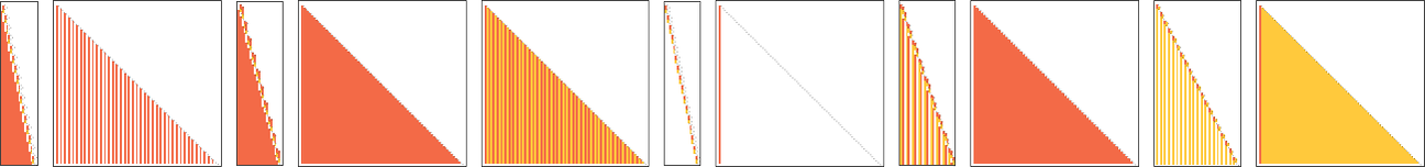
one might think they would be simple enough to have shorter runtimes. But in fact in the one-sided setup their behavior is basically identical to our original machine.
OK, but what about
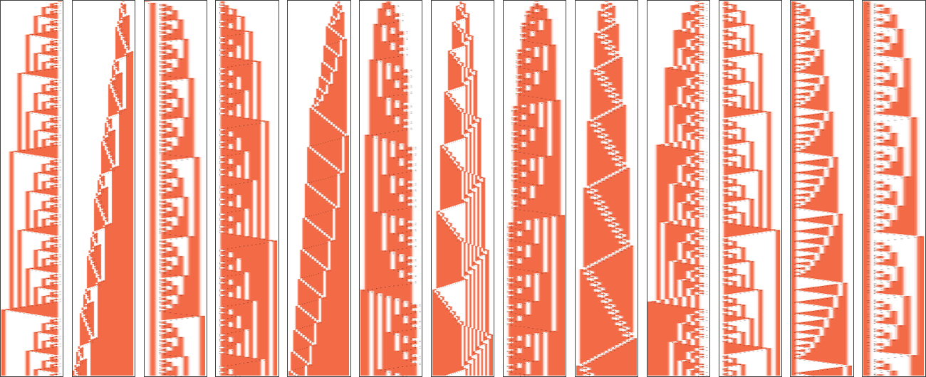
We’ve been talking a lot about how fast Turing machines can compute functions. But what can we say about what functions they compute? With appropriate encoding of inputs and decoding of outputs, we know that (essentially by definition) any computable function can be computed by some Turing machine. But what about the simple Turing machines we’ve been using here? And what about “without encodings”?
The way we’ve set things up, we’re taking both the input and the output to our Turing machines to be the sequences of values on their tapes—and we’re interpreting these values as digits of integers. So that means we can think of our Turing machines as defining functions from integers to integers. But what functions are they?
Here are two
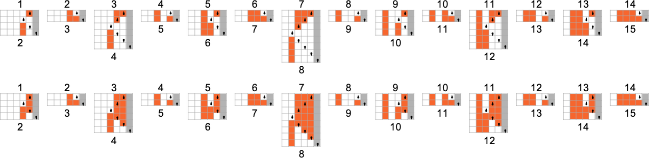
There are a total of 17
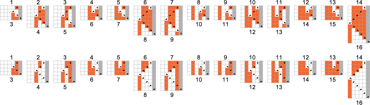
Still, for
If we restrict ourselves to even inputs, then we can compute
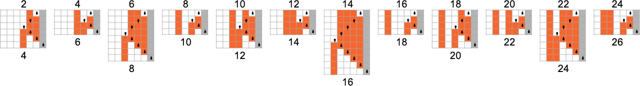
Similarly, there are
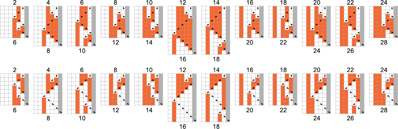
What about other “mathematically simple” functions, say
We’ve already seen a variety of examples where our Turing machines can be interpreted as evaluating bitwise functions of their inputs. A more minimal case would be something like a single bitflip—and indeed there is an
To be able to flip a higher-order digit, one needs a Turing machine with more states. There are two

And in general—as these pictures suggest—flipping the mth bit can be done with a Turing machine with at least
What about Turing machines that compute periodic functions? Strict (nontrivial) periodicity seems difficult to achieve. But here, for example, is an
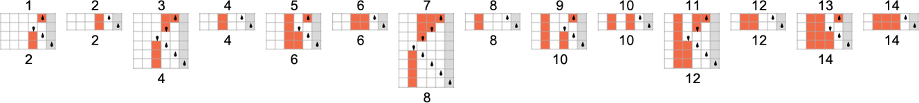
With both
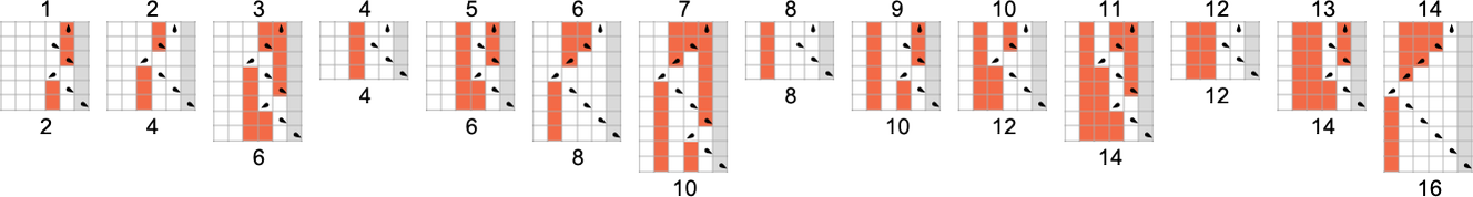
Another thing one might ask is whether one Turing machine can emulate another. And indeed that’s what we see happening—very directly—whenever one Turing machine computes the same function as another.
(We also know that there exist universal Turing machines—the simplest having
Computational irreducibility has been central to much of the science I’ve done in the past four decades or so. And indeed it’s guided our intuition in much of what we’ve been exploring here. But the things we’ve discussed now also allow us to take an empirical look at the core phenomenon of computational irreducibility itself.
Computational irreducibility is ultimately about the idea that there can be computations where in effect there is no shortcut: there is no way to systematically find their results except by running each of their steps. In other words, given an irreducible computation, there’s basically no way to come up with another computation that gives the same result, but in fewer steps. Needless to say, if one wants to tighten up this intuitive idea, there are lots of detailed issues to consider. For example, what about just using a computational system that has “bigger primitives”? Like many other foundational concepts in theoretical science, it’s difficult to pin down exactly how one should set things up—so that one doesn’t either implicitly assume what one’s trying to explain, or so restrict things that everything becomes essentially trivial.
But using what we’ve done here, we can explore a definite—if restricted—version of computational irreducibility in a very explicit way. Imagine we’re computing a function using a Turing machine. What would it mean to say that that function—and the underlying behavior of the Turing machine that computes it—is computationally irreducible? Essentially it’s that there’s no other faster way to compute that function.
But if we restrict ourselves to computation by a certain size of Turing machine, that’s exactly what we’ve studied at great length here. And, for example, whenever we have what we’ve called an “isolate” Turing machine, we know that no other Turing machine of the same size can compute the same function. So that means one can say that the function is computationally irreducible with respect to Turing machines of the given size.
How robust is such a notion? We’ve seen examples above where a given function can be computed, say, only in exponential time by an
But the important point here is that we can already see a restricted version of computational irreducibility just by looking explicitly at Turing machines of a given size. And this allows us to get concrete results about computational irreducibility, or at least about this restricted version of it.
One of the remarkable discoveries in looking at lots of kinds of systems over the years has been just how common the phenomenon of computational irreducibility seems to be. But usually we haven’t had a way to rigorously say that we’re seeing computational irreducibility in any particular case. All we typically know is that we can’t “visually decode” what’s going on, nor can particular methods we try. (And, yes, the fact that a wide variety of different methods almost always agree about what’s “compressible” and what’s not encourages our conclusions about the presence of computational irreducibility.)
In looking at Turing machines here, we’re often seeing “visual complexity”, not so much in the detailed—often ponderous—behavior with a particular initial condition, but more, for example, in what we get by plotting function values against inputs. But now we have a more rigorous—if restricted—test for computational irreducibility: we can ask whether the function that’s being computed is irreducible with respect to this size of Turing machine, or, typically equivalently, whether the Turing machine we’re looking at is an isolate.
So now we can, for example, explore how common irreducibility defined in this way might be. Here are results for some of the classes of small Turing machines we’ve studied above:
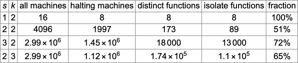
And what we see is that—much like our impression from computational systems like cellular automata—computational irreducibility is indeed very common among small Turing machines, where now we’re using our rigorous, if restricted, notion of computational irreducibility.
(It’s worth commenting that while “global” features of Turing machines—like the functions they compute—may be computationally irreducible, there can still be lots of computational reducibility in their more detailed properties. And indeed what we’ve seen here is that there are plenty of features of the behavior of Turing machines—like the back-and-forth motion of their heads—that look visually simple, and that we can expect to compute in dramatically faster ways than just running the Turing machine itself.)
So far, we’ve made a fairly extensive study of ordinary, deterministic (“single-way”) Turing machines. But the P vs. NP question is about comparing the capabilities of such deterministic Turing machines with the capabilities of nondeterministic—or multiway—Turing machines.
An ordinary (deterministic) Turing machine has a rule such as
that specifies a unique sequence of successive configurations for the Turing machine
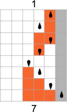
which we can represent as:
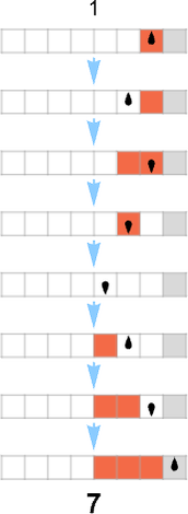
A multiway Turing machine, on the other hand, can have multiple rules, such as
which are applied in all possible ways to generate a whole multiway graph of successive configurations for the Turing machine
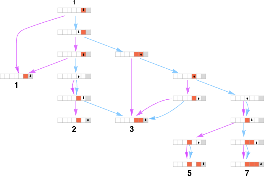
where we have indicated edges in the multiway graph associated with the application of each rule respectively by ![]() and
and ![]() , and where identical Turing machine configurations are merged.
, and where identical Turing machine configurations are merged.
Just as we have done for ordinary (deterministic) Turing machines, we take multiway Turing machines to reach a halting configuration whenever the head goes further to the right than it started—though now this may happen on multiple branches—so that the Turing machine in effect can generate multiple outputs.
With the way we have set things up, we can think of an ordinary (deterministic) Turing machine as taking an input i and giving as output some value f[i] (where that value might be undefined if the Turing machine doesn’t halt for a given i). In direct analogy, we can think of a multiway Turing machine as taking an input i and giving potentially a whole collection of corresponding outputs:
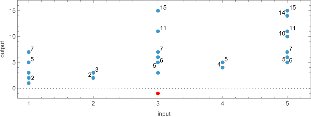
Among the immediate complications is the fact that the machine may not halt, at least on some branches—as happens for input 3 here, indicated by a red dot in the plot above:
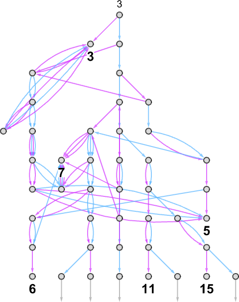
(In addition, we see that there can be multiple paths that lead to a given output, in effect defining multiple runtimes for that output. There can also be cycles, but in defining “runtimes” we ignore these.)
When we construct a multiway graph we are effectively setting up a representation for all possible paths in the evolution of a (multiway) system. But when we talk about nondeterministic evolution we are typically imagining that just a single path is going to be followed, but we don’t know which.
Let’s say that we have a multiway Turing machine that for every given input generates a certain set of outputs. If we were to pick just one of the outputs from each of these sets, we would effectively in each case be picking one path in the multiway Turing machine. Or, in other words, we would be “doing a nondeterministic computation”, or in effect getting output from a nondeterministic Turing machine.
As an example, let’s take our multiway Turing machine from above. Here is an example of how this machine—thought of as a nondeterministic Turing machine—can generate a certain sequence of output values:
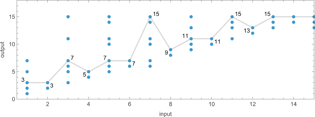
Each of these output values is achieved by following a certain path in the multiway graph obtained with each input:
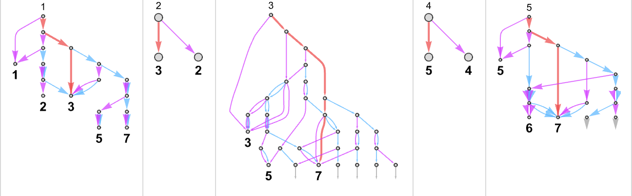
Keeping only the path taken (and including the underlying Turing machine configuration) this represents how each output value was “derived”:
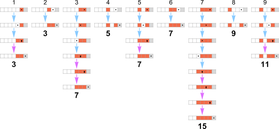
The length of the path can then be thought of as the runtime required for the nondeterministic Turing machine to reach the output value. (When there are multiple paths to a given output value, we’ll typically consider “the runtime” to be the length of the shortest of these paths.) So now we can summarize the runtimes from our example as follows:
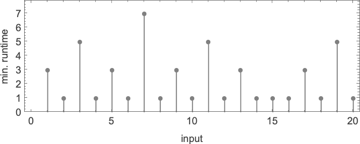
The core of the P vs. NP problem is to compare the runtime for a particular function obtained by deterministic and nondeterministic Turing machines.
So, for example, given a deterministic Turing machine that computes a certain function, we can ask whether there is a nondeterministic Turing machine which—if you picked the right branch—can compute that same function, but faster.
In the case of the example above, there are two possible underlying Turing machine rules indicated by ![]() and
and ![]() . For each input we can choose at each step a different rule to apply in order to get to the output:
. For each input we can choose at each step a different rule to apply in order to get to the output:
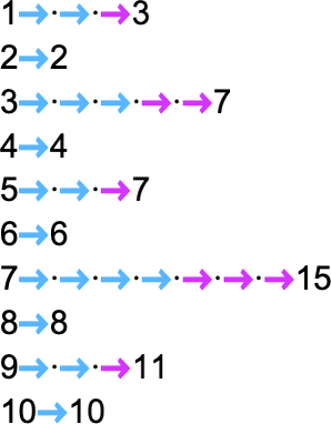
The possibility of using different rules at different steps in effect allows much more freedom in how our computation can be done. The P vs. NP question concerns whether this freedom allows one to fundamentally speed up the computation of a given function.
But before we explore that question further, let’s take a look at what multiway (nondeterministic) Turing machines typically do; in other words, let’s study their ruliology.
As our first example of doing ruliology for multiway Turing machines, let’s consider the case of pairs of

Sometimes, as in machine {1,9}, there turns out to be a unique output value for every input:
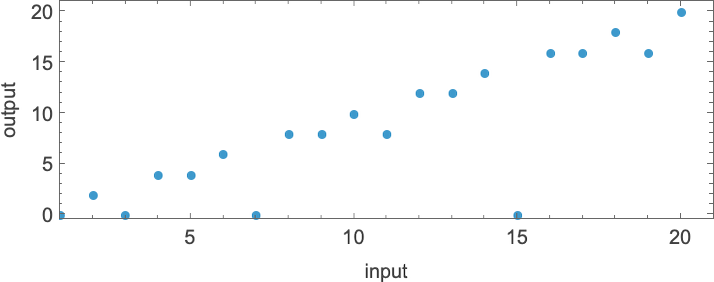
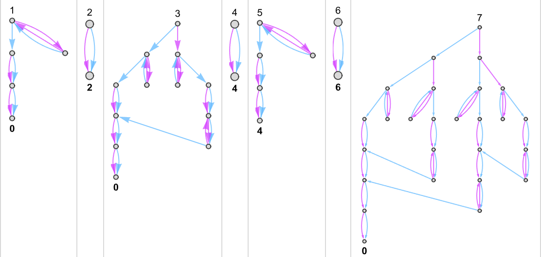
Sometimes, as in machine {5,9}, there is usually a unique value, but sometimes not:
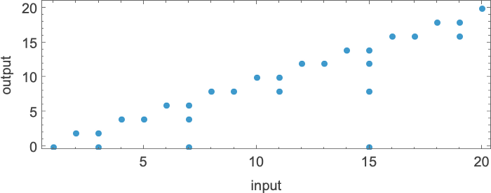
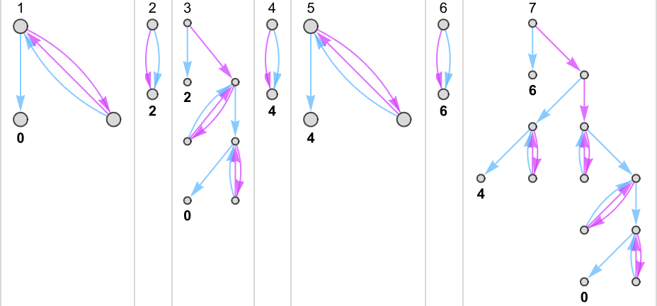
Something similar happens with {3,7}:
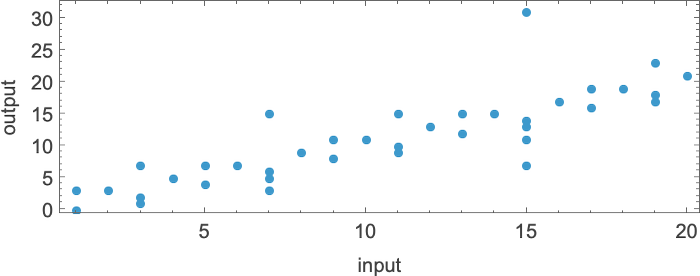
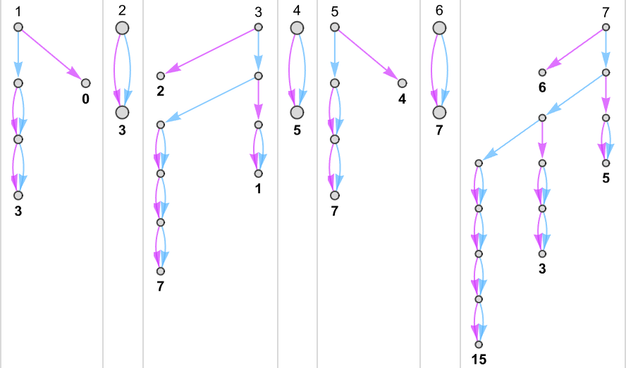
There are cases—like {1,3}—where for some inputs there’s a “burst” of possible outputs:
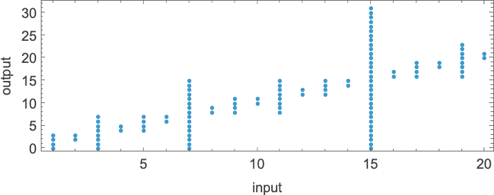
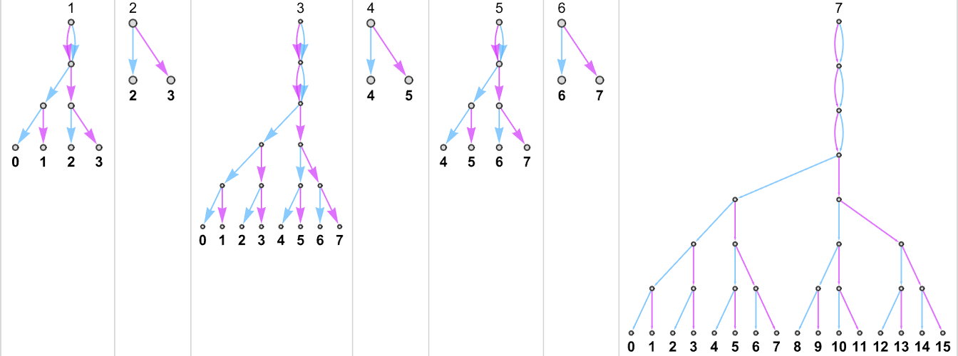
There are also plenty of cases where for some inputs
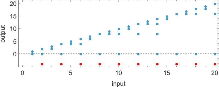
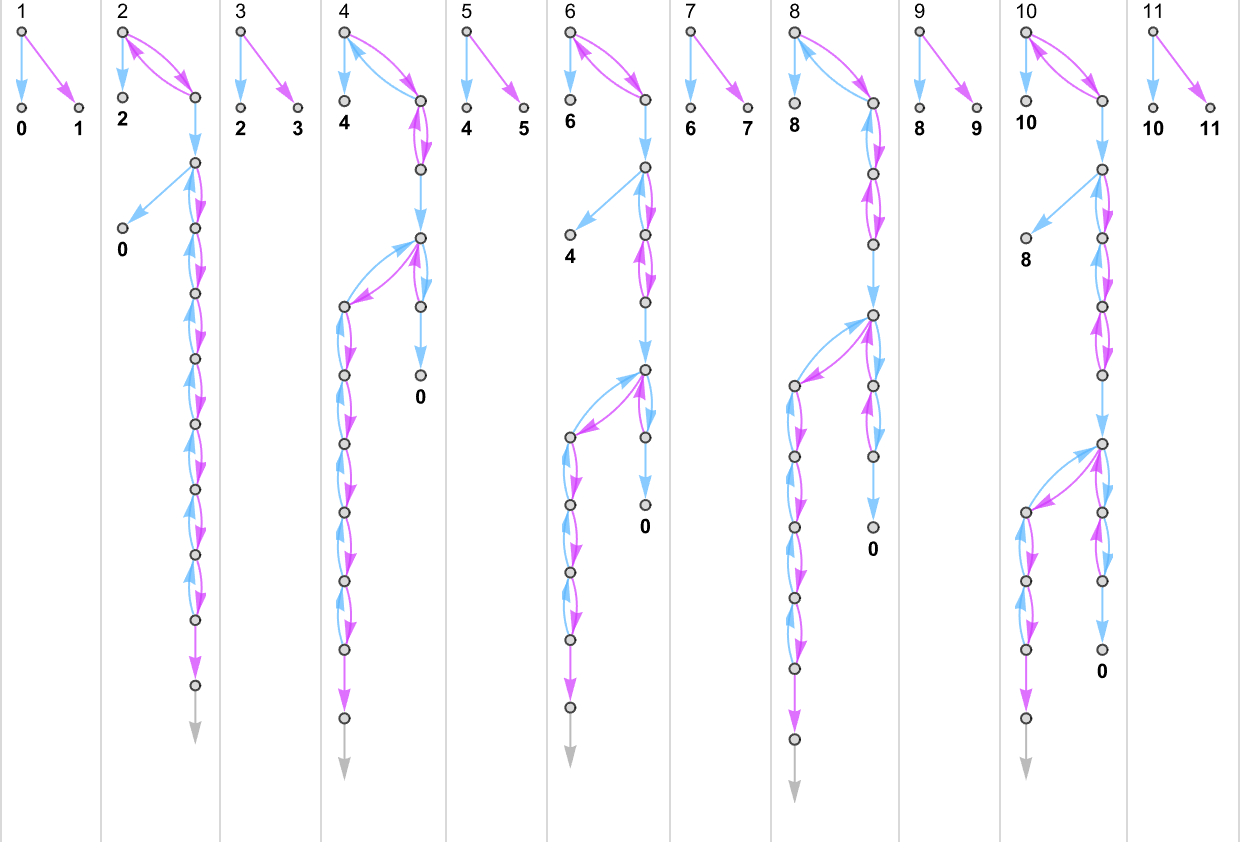
or for all inputs, there are branches that do not halt:
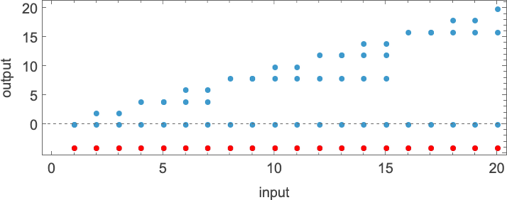
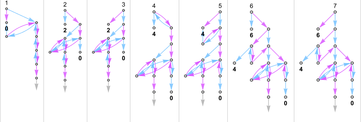
What about runtimes? Well, for each possible output in a nondeterministic Turing machine, we can see how many steps it takes to reach that output on any branch of the multiway graph, and we can consider that minimum number to be the “nondeterministic runtime” needed to compute that output.
It’s the quintessential setup for NP computations: if you can successfully guess what branch to follow, you can potentially get to an answer quickly. But if you have to explicitly check each branch in turn, that can be a slow process.
Here’s an example showing possible outputs and possible runtimes for a sequence of inputs for the {3,7} nondeterministic machine
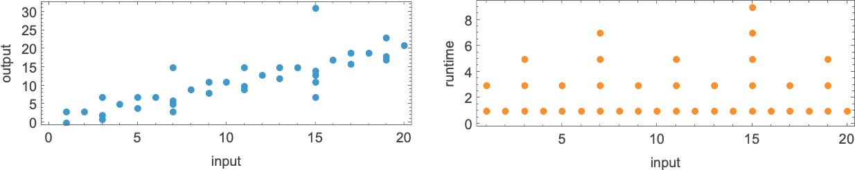
or, combined in 3D:
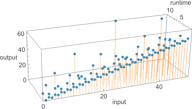
So what functions can a nondeterministic machine like this “nondeterministically” generate? For each input we have to pick one of the possible corresponding (“multiway”) outputs. And in effect the possible functions correspond to possible “threadings” through these values
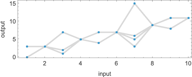
or:
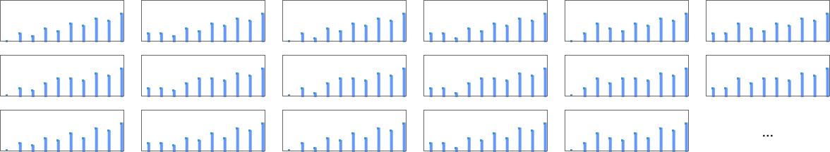
To each function one can then associate a “nondeterministic runtime” for each output, here:
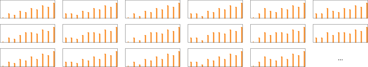
We’ve seen how a nondeterministic machine can in general generate multiple functions, with each output from the function being associated with a minimum (“nondeterministic”) runtime. But how do the functions that a particular nondeterministic machine can generate compare with the functions that deterministic machines can generate? Or, put another way, given a function that a nondeterministic machine can generate (or “compute”), what deterministic machine is required to compute the same function?
Let’s look at the
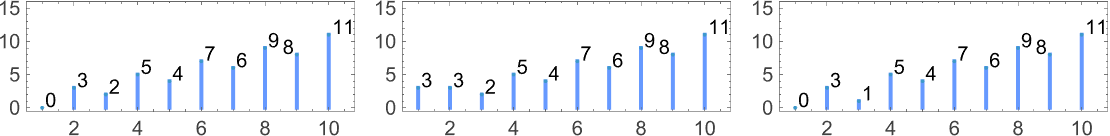
Can we find a deterministic ![]() ) branch in the multiway system
) branch in the multiway system
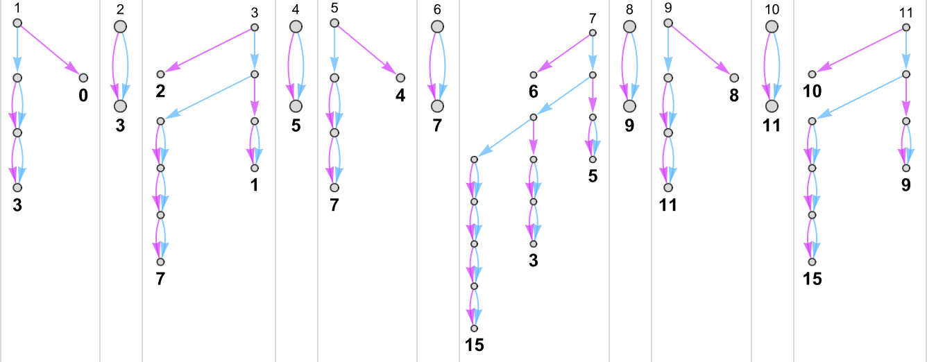
so that it inevitably gives the same results as deterministic machine 3.
But (apart from the other trivial case based on following “machine 7” branches) none of the other functions we can generate from this nondeterministic machine can be reproduced by any
What about
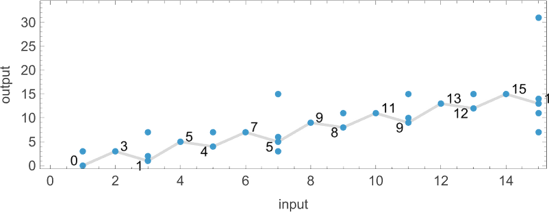
And here are the paths through the multiway graphs for that machine that get to these values
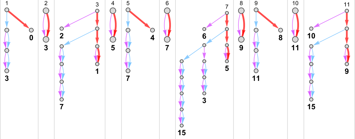
with the “paths on their own” being
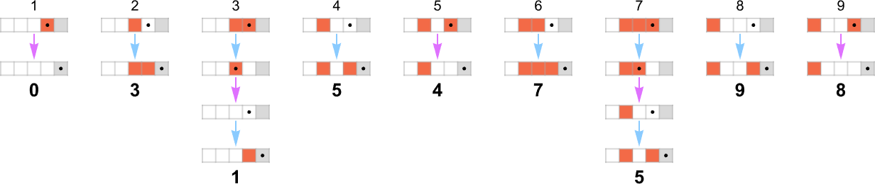
yielding “nondeterministic runtimes”:
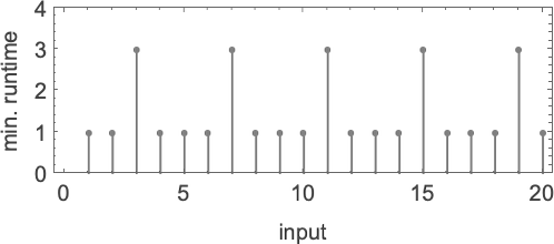
This is how the deterministic
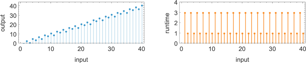
Here are the pair of underlying rules for the nondeterministic machine
and here is the deterministic machine that reproduces a particular function it can generate:
This example is rather simple, and has the feature that even the deterministic machine always has a very small runtime. But now the question we can ask is whether a function that takes a deterministic machine of a certain class a certain time to compute can be computed in a smaller time if its results are “picked out of” a nondeterministic machine.
We saw above that
But what about a nondeterministic machine? How fast can this be?
It turns out that there are 15 nondeterministic machines based on pairs of
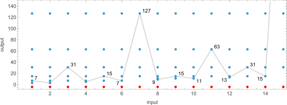
Here are the paths within the multiway graph for the nondeterministic machine that are sampled to generate the deterministic Turing machine result:
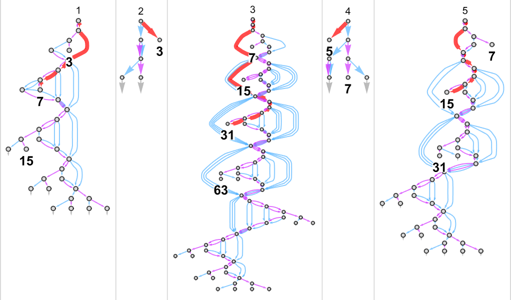
And here are these “paths on their own”:
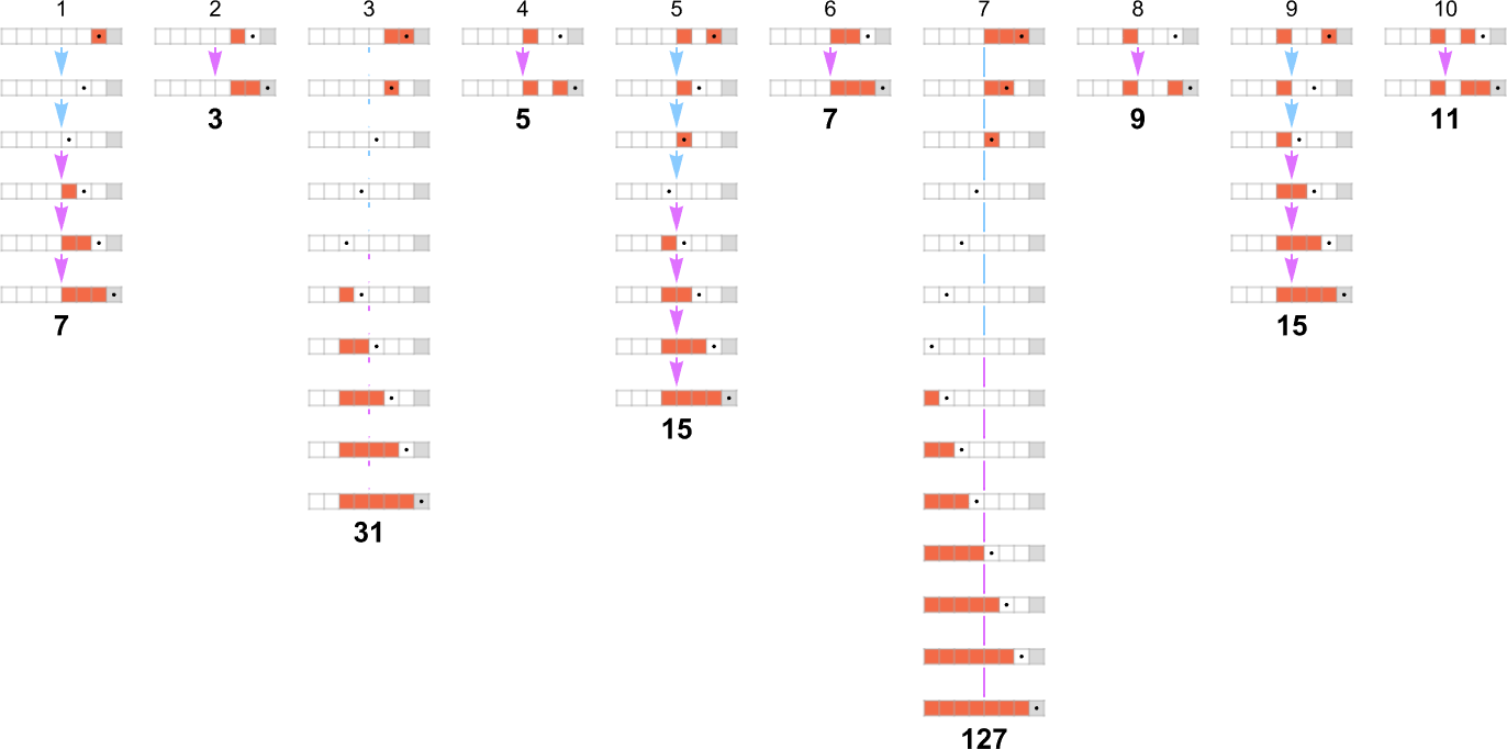
We can compare these with the computations needed in the deterministic machine:
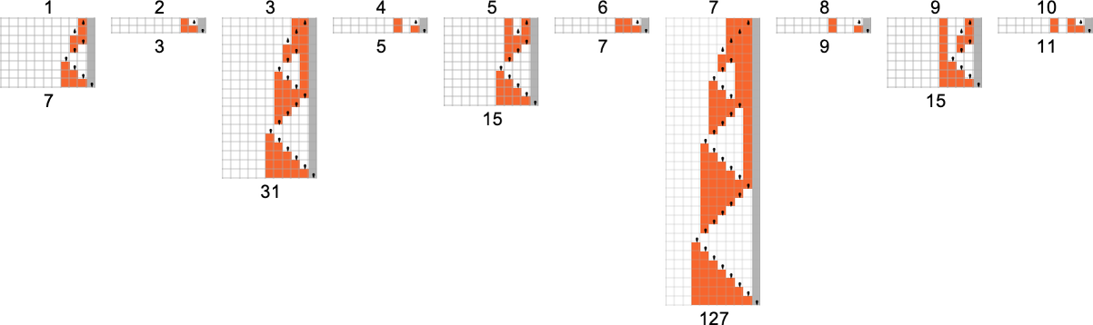
With our rendering, the lengths of the nondeterministic paths might look longer. But in fact they are considerably shorter, as we see by plotting them (in orange) along with the deterministic runtimes (in gray):
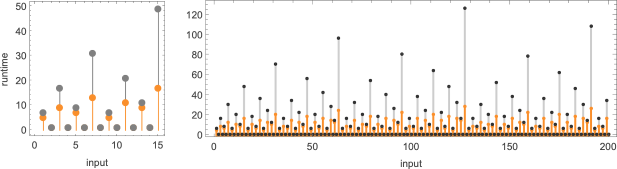
Looking now at the worst-case runtimes for inputs of size n, we get:
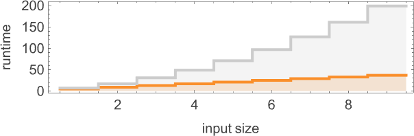
For the deterministic machine we found above for input size n, this worst-case runtime is given by:
But now the runtime in the nondeterministic machine turns out to be:
In other words, we’re seeing that nondeterminism makes it substantially faster to compute this particular function—at least by small Turing machines.
In a deterministic machine, it’s always the same underlying rule that’s applied at each step. But in a nondeterministic machine with the setup we’re using, we’re independently choosing one of two different rules to apply at each step. The result is that for every function value we compute, we’re making a sequence of choices:
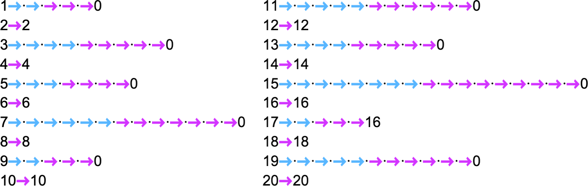
And the core question that underlies things like the P vs. NP problem is how much advantage the freedom to make these choices conveys—and whether, for example, it allows us to “nondeterministically” compute in polynomial time what takes more than polynomial (say, exponential) time to compute deterministically.
As a first example, let’s look at the function computed by the ![]() – 1
– 1
Well, it turns out that the
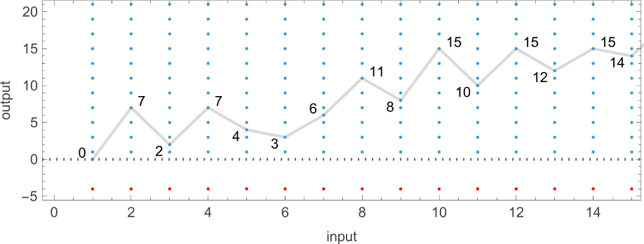
And indeed, while the deterministic machine takes exponentially increasing runtime, the nondeterministic machine has a runtime that quickly approaches the fixed constant value of 5:
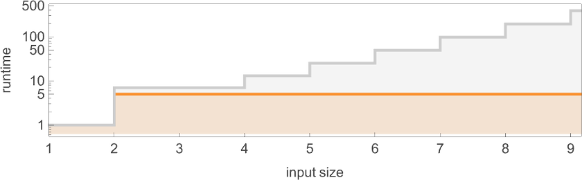
But is this somehow trivial? As the plot above suggests, the nondeterministic machine (at least eventually) generates all possible odd output values (and for even input i, also generates
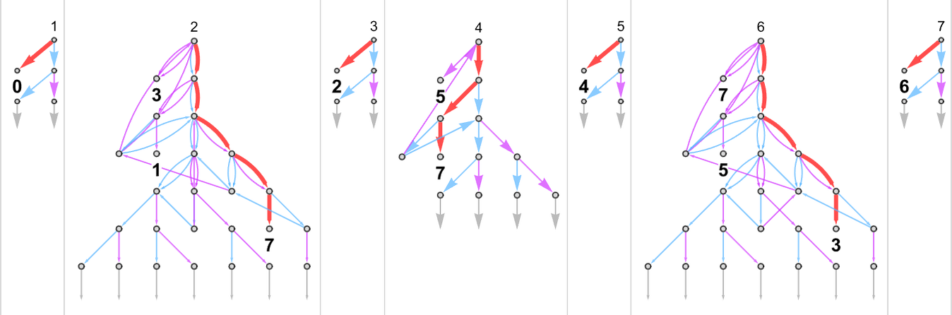
What makes the runtime end up being constant, however, is that in this particular case, the output f[i] is always close to i (in fact,
There are actually no fewer than
And while all of them are in a sense straightforward in their operation, they illustrate the point that even when a function requires exponential time for a deterministic Turing machine, it can require much less time for a nondeterministic machine—and even a nondeterministic machine that has a much smaller rule.
What about other cases of functions that require exponential time for deterministic machines? The functions computed by the
Something slightly different happens with
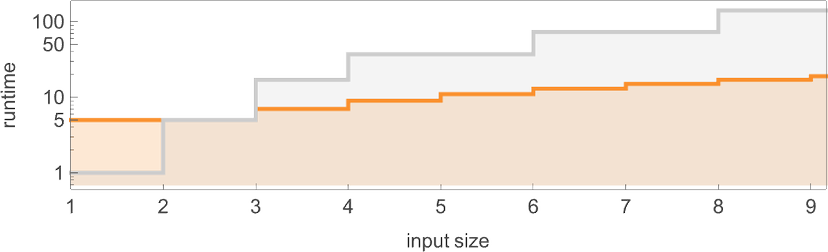
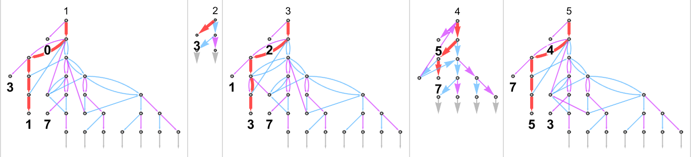
A deterministic Turing machine has a single, definite rule that’s applied at each step. In the previous sections we’ve explored what’s in a sense a minimal case of nondeterminism in Turing machines—where we allow not just one, but two different possible rules to be applied at each step. But what if we increase the nondeterminism—say by allowing more possible rules at each step?
We’ve seen that there’s a big difference between determinism—with one rule—and even our minimal case of nondeterminism, with two rules. But if we add in, say, a third rule, it doesn’t seem to typically make any qualitative difference. So what about the limiting case of adding in all conceivable rules?
We can think of what we get as an “everything machine”—a machine that has every possible rule case for any possible Turing machine, say for
Running this “everything machine” for one step starting with input 1 we get:
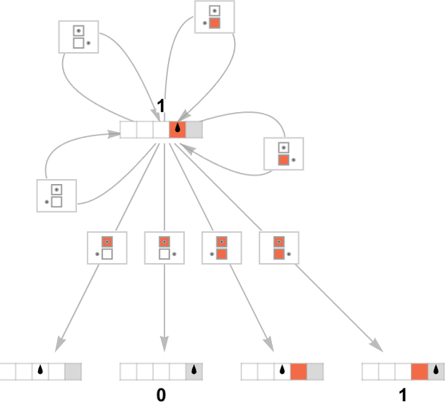
Four of the rule cases just lead back to the initial state. Then of the other four, two lead to halting states, and two do not. Dropping self-loops, going another couple of steps, and using a different graph rendering, we see that outputs 2 and 3 now appear:
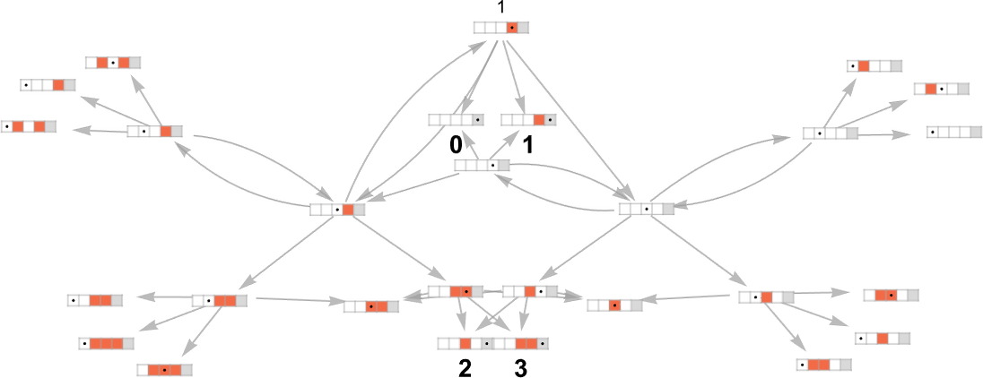
Here are the results for input 2:
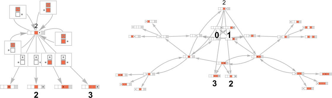
So where can the “everything machine” reach, and how long does it take? The answer is that from any input i it can eventually reach absolutely any output value j. The minimum number of steps required (i.e. the minimum path length in the multiway graph) is just the absolute lower bound that we found for runtimes in deterministic machines above:
Starting with input 1, the nondeterministic runtime to reach output j is then
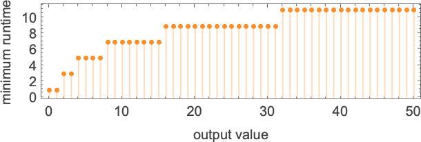
which grows logarithmically with output value, or linearly with output size.
So what this means is that the “everything machine” lets one nondeterministically go from a given input to a given output in the absolutely minimum number of steps structurally possible. In other words, with enough nondeterminism every function becomes nondeterministically “easy to compute”.
An important feature of the “everything machine” is that we can think of it as being a fragment of the ruliad. The full ruliad—which appears at the foundations of physics, mathematics and much more—is the entangled limit of all possible computations. There are many possible bases for the ruliad; Turing machines are one. In the full ruliad, we’d have to consider all possible Turing machines, with all possible sizes. The “everything machine” we’ve been discussing here gives us just part of that, corresponding to all possible Turing machine rules with a specific number of states and colors.
In representing all possible computations, the ruliad—like the “everything machine”—is maximally nondeterministic, so that it in effect includes all possible computational paths. But when we apply the ruliad in science (and even mathematics) we are interested not so much in its overall form as in particular slices of it which are sampled by observers that, like us, are computationally bounded. And indeed in the past few years it’s become clear that there’s a lot to say about the foundations of many fields by thinking in this way.
And one feature of computationally bounded observers is that they’re not maximally nondeterministic. Instead of following all possible paths in the multiway system, they tend to follow specific paths or bundles of paths—for example reflecting the single thread of experience that characterizes our human perception of things. So—when it comes to observers—the “everything machine” is somehow too nondeterministic. An actual (computationally bounded) observer will be concerned with one or just a few “threads of history”. In other words, if we’re interested in slices of the ruliad that observers will sample, what will be relevant is not so much the “everything machine” but rather deterministic machines, or at most machines with the kind of limited nondeterminism that we’ve studied the past few sections.
But just how does what the “everything machine” can do compare with what all possible deterministic machines can do? In some ways, this is a core question in the comparison between determinism and nondeterminism. And it’s straightforward to start studying it empirically.
For example, here are successive steps in the multiway graph for the (
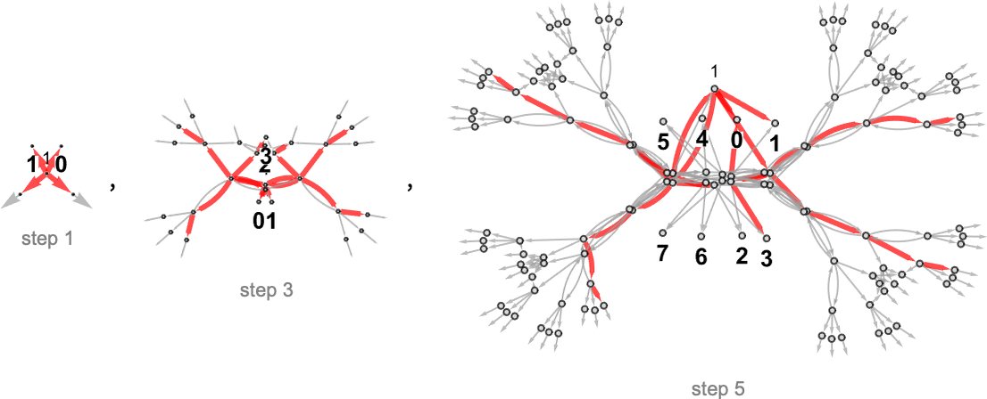
In a sense these pictures illustrate the “reach” of deterministic vs. nondeterministic computation. In this particular case, with
For
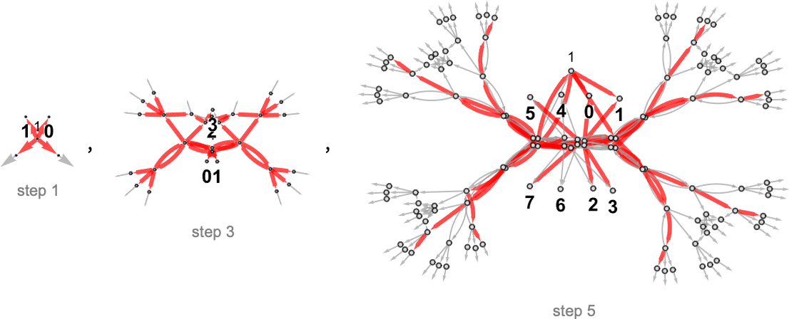
and the values that can be reached by deterministic machines are:
But how long does it take to reach these values? This shows as dots the possible (deterministic) runtimes; the filling represents the minimum (nondeterministic) runtimes for the “everything machine”:
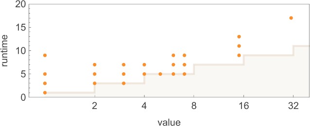
The most dramatic outlier occurs with value 31, which is reached deterministically only by machine 1447, in 15 steps, but which can be reached in 9 (nondeterministic) steps by the “everything machine”:
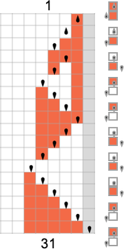
For
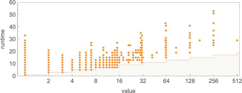

The P vs. NP question asks whether every computation that can be done by any nondeterministic Turing machine with a runtime that increases at most polynomially with input size can also be done by some deterministic Turing machine with a runtime that also increases at most polynomially. Or, put more informally, it asks whether introducing nondeterminism can fundamentally speed up computation.
In its full form, this is an infinite question, that talks about limiting behavior over all possible inputs, in all possible Turing machines. But within this infinite question, there are definite, finite subquestions we can ask. And one of the things we’ve done here is in effect to explore some of these questions in an explicit, ruliological way. Looking at these finite subquestions won’t in any direct way be able to resolve the full P vs. NP question.
But it can give us important intuition about the P vs. NP question, and what some of the difficulties and subtleties involved in it are. When one analyzes specific, constructed algorithms, it’s common to see that their runtimes vary quite smoothly with input size. But one of the things we’ve seen here is that for arbitrary Turing machines “in the wild”, it’s very typical for the runtimes to jump around in complicated ways. It’s also not uncommon to see dramatic outliers that occur only for very specific inputs.
If there was just one outlier, then in the limit of arbitrarily large input size it would eventually become irrelevant. But what if there were an unending sequence of outliers, of unpredictable sizes at unpredictable positions? Ultimately we expect all sorts of computational irreducibility, which in the limit can make it infinitely difficult to determine in any particular case the limiting behavior of the runtime—and, for example, to find out if it’s growing like a polynomial or not.
One might imagine, though, that if one looked at enough inputs, enough Turing machines, etc. then somehow any wildness would get in some way averaged out. But our ruliological results don’t encourage that idea. And indeed they tend to show that “there’s always more wildness”, and it’s somehow ubiquitous. One might have imagined that computational irreducibility—or undecidability—would be sufficiently rare that it wouldn’t affect investigations of “global” questions like the P vs. NP one. But our results suggest that, to the contrary, there are all sorts of complicated details and “exceptions” that seem to get in the way of general conclusions.
Indeed, there seem to be issues at every turn. Some are related to unexpected behavior and outliers in runtimes. Some are related to the question of whether a particular machine ever even halts at all for certain inputs. And yet others are related to taking limits of sizes of inputs versus sizes of Turing machines, or amounts of nondeterminism. What our ruliological explorations have shown is that such issues are not obscure corner cases; rather they are generic and ubiquitous.
One has the impression, though, that they are more pronounced in deterministic than in nondeterministic machines. Nondeterministic machines in some sense “aggregate” over paths, and in doing so, wash out the “computational coincidences” which seem ubiquitous in determining the behavior of deterministic machines.
Certainly the specific experiments we’ve done on machines of limited size do seem to support the idea that there are indeed computations that can be done quickly by a nondeterministic machine, but for which in deterministic machines there are for example at least occasional large runtime outliers, which imply longer general runtimes.
I had always suspected that the P vs. NP question would ultimately get ensnared in issues of computational irreducibility and undecidability. But from our explicit ruliological explorations we get an explicit sense of how this can happen. Will it nevertheless ultimately be possible to resolve the P vs. NP question with a finite mathematical-style proof based, say, on standard mathematical axioms? The results here make me doubt it.
Yes, it will be possible to get at least certain restricted global results—in effect by “mining” pockets of computational reducibility. And, as we already know from what we have seen repeatedly here, it’s also possible to get definite results for, say, specific (ultimately finite) classes of Turing machines.
I’ve only scratched the surface here of the ruliological results that can be found. In some cases to find more just requires expending more computer time. In other cases, though, we can expect that new methodologies, particularly around “bulk” automated theorem proving, will be needed.
But what we’ve seen here already makes it clear that there is much to be learned by ruliological methods about questions of theoretical computer science—P vs. NP among them. In effect, we’re seeing that theoretical computer science can be done not only “purely theoretically”—say with methods from traditional mathematics—but also “empirically”, finding results and developing intuition by doing explicit computational experiments and enumerations.
My efforts on what I now call ruliology started at the beginning of the 1980s, and in the early years I almost exclusively studied cellular automata. A large part of the reason was just that these were the first types of simple programs I’d investigated, and in them I had made a series of discoveries. I was certainly aware of Turing machines, but viewed them as less connected than cellular automata to my goal of studying actual systems in nature and elsewhere—though ultimately theoretically equivalent.
It wasn’t until 1991, when I started systematically studying different types of simple programs as I embarked on my book A New Kind of Science that I actually began to do simulations of Turing machines. (Despite their widespread use in theoretical science for more than half a century, I think almost nobody else—from Alan Turing on—had ever actually simulated them either.) At first I wasn’t particularly enamored of Turing machines. They seemed a little less elegant than mobile automata, and had much less propensity to show interesting and complex behavior than cellular automata.
Towards the end of the 1990s, though, I was working to connect my discoveries in what became A New Kind of Science to existing results in theoretical computer science—and Turing machines emerged as a useful bridge. In particular, as part of the final chapter of A New Kind of Science—“The Principle of Computational Equivalence”—I had a section entitled “Undecidability and Intractability”. And in that section I used Turing machines as a way to explore the relation of my results to existing results on computational complexity theory.
And it was in the process of that effort that I invented the kind of one-sided Turing machines I’ve used here:

I concentrated on the s = 2, k = 2 machines (for some reason I never looked at s = 1, k = 2), and found classes of machines that compute the same function—sometimes at different speeds:

And even though the computers I was using at the time were much slower than the ones I use today, I managed to extend what I was doing to s = 3, k = 2. At every turn, though, I came face to face with computational irreducibility and undecidability. I tried quite hard do things like resolve the exact number of distinct functions for

Nearly three decades later, I think I finally have the exact number. (Note that some of the details from A New Kind of Science are also different from what I have here, because in A New Kind of Science I included partial functions in my enumeration; here I’m mostly insisting on total functions, that halt and give a definite result for all inputs.)
After A New Kind of Science was released in 2002, I made another foray into Turing machines in 2007, putting up a prize on the fifth anniversary of the book for a proof (or refutation) of my suspicion that s = 2, k = 3 machine 596440 was capable of universal computation. The prize was soon won, establishing this machine as the very simplest universal Turing machine:

Many years passed. I occasionally suggested projects on Turing machines to students at the summer research program we started in 2003 (more on that later…). And I participated in celebrations of Alan Turing’s centenary in 2012. Then in 2020 we announced the Wolfram Physics Project—and I looked at Turing machines again, now as an example of a computational system that could be encoded with hypergraph rewriting, and studied using physics-inspired causal graphs, etc.:

Less than two months after the launch of our Physics Project I was studying what I now call the ruliad—and I decided to use Turing machines as a model for it:

A crucial part of this was the idea of multiway Turing machines:

I’d introduced multiway systems in A New Kind of Science, and had examples close to multiway Turing machines in the book. But now multiway Turing machines were more central to what I was doing—and in fact I started studying essentially what I’ve here called the “everything machine” (though the details were different, because I wasn’t considering Turing machines that can halt):

I also started looking at the comparison between what can be reached deterministically and nondeterministically—and discussed the potential relation of this to the P vs. NP question:

By the next year, I was expanding my study of multiway systems, and exploring many different examples—with one of them being multiway Turing machines:

Soon I realized that the general approach I was taking could be applied not only to the foundations of physics, but also to foundations of other fields. I studied the foundations of mathematics, of thermodynamics, of machine learning and of biology. But what about the foundations of theoretical computer science?
Over the years, I’d explored the ruliology of many kinds of systems studied in theoretical computer science—doing deep dives into combinators for their centenary in 2020, as well as (last year) into lambdas. In all these investigations, I was constantly seeing concrete versions of phenomena discussed in theoretical computer science—even though my emphasis tended to be different. But I was always curious what one might be able to say about central questions in theoretical computer science—like P vs. NP.
I had imagined that the principal problem in doing an empirical investigation of something like P vs. NP would just be to enumerate enough cases. But when I got into it, I realized that the shadow of computational irreducibility loomed even larger than I’d imagined—and that even within particular cases it could be irreducibly difficult to figure out what one needed to know about their behavior.
Fairly late in the project I was trying to look up some “conventional wisdom” about NP problems. Most of it was couched in rather traditional mathematical terms, and didn’t seem likely to have too much to say about what I was doing. But then I found a paper entitled “Program-size versus Time Complexity: Slowdown and Speed-up Phenomena in the Micro-cosmos of Small Turing Machines”—and I was excited to see that it was following up on what I’d done in A New Kind of Science, and doing ruliology. But then I realized: the lead author of the paper, Joost Joosten, had been an (already-a-professor) student at our summer program in 2009, and I’d in fact suggested the original version of the project (though the paper had taken it further, and in some slightly different directions than I’d anticipated).
Needless to say, what I’ve now done here raises a host of new questions, which can now be addressed by future projects done at our summer programs, and beyond….
Note: For general historical background see my related writings from 2002 and 2021.
Thanks to Willem Nielsen, Nik Murzin and Brian Mboya of the Wolfram Institute for extensive help. Thanks also to Wolfram Institute affiliate Anneline Daggelinckx, as well as to Richard Assar and Pavel Hajek of the Wolfram Institute for additional help. Work at the Wolfram Institute on this project was supported in part by the John Templeton Foundation.
Additional input on the project was provided by Lenore & Manuel Blum, Christopher Gilbert, Josh Grochow, Don Knuth and Michael Sun. Matthew Szudzik also contributed relevant work in 1999 during the development of A New Kind of Science.
2026-01-13 07:05:20

Ruliology is taking off! And more and more people are talking about it. But what is ruliology? Since I invented the term, I decided I should write something to explain it. But then I realized: I actually already wrote something back in 2021 when I first invented the term. What I wrote back then was part of something longer. But here now is the part that explains ruliology:

If one sets up a system to follow a particular set of simple rules, what will the system do? Or, put another way, how do all those simple programs out there in the computational universe of possible programs behave?
These are pure, abstract questions of basic science. They’re questions one’s led to ask when one’s operating in the computational paradigm that I describe in A New Kind of Science. But at some level they’re questions about the specific science of what abstract rules (that we can describe as programs) do.
What is that science? It’s not computer science, because that would be about programs we construct for particular purposes, rather than ones that are just “out there in the wilds of the computational universe”. It’s not (as such) mathematics, because it’s all about “seeing what rules do” rather than finding frameworks in which things can be proved. And in the end, it’s clear it’s actually a new science—that’s rich and broad, and that I, at least, have had the pleasure of practicing for forty years.
But what should this science be called? I’ve wondered about this for decades. I’ve filled so many pages with possible names. Could it be based on Greek or Latin words associated with rules? Those are arch- and reg-: very well-trafficked roots. What about words associated with computation? That’d be logis- or calc-. None of these seem to work. But—in something akin to the process of metamodeling—we can ask: What is the essence of what we want to communicate in the word?
It’s all about studying rules, and what their consequences are. So why not the simple and obvious “ruliology”? Yes, it’s a new and slightly unusual-sounding word. But I think it does well at communicating what this science that I’ve enjoyed for so long is about. And I, for one, will be pleased to call myself a “ruliologist”.
But what is ruliology really about? It’s a pure, basic science—and a very clean and precise one. It’s about setting up abstract rules, and then seeing what they do. There’s no “wiggle room”. No issue with “reproducibility”. You run a rule, and it does what it does. The same every time.
What does the rule 73 cellular automaton starting from a single black cell do? What does some particular Turing machine do? What about some particular multiway string substitution system? These are specific questions of ruliology.
At first you might just do the computation, and visualize the result. But maybe you notice some particular feature. And then you can use whatever methods it takes to get a specific ruliological result—and to establish, for example, that in the rule 73 pattern, black cells appear only in odd-length blocks.
Ruliology tends to start with specific cases of specific rules. But then it generalizes, looking at broader ranges of cases for a particular rule, or whole classes of rules. And it always has concrete things to do—visualizing behavior, measuring specific features, and so on.
But ruliology quickly comes face to face with computational irreducibility. What does some particular case of some particular rule eventually do? That may require an irreducible amount of computational effort to find out—and if one insists on knowing what amounts to a general truly infinite-time result, it may be formally undecidable. It’s the same story with looking at different cases of a rule, or different rules. Is there any case that does this? Or any rule that does it?
What’s remarkable to me—even after 40 years of ruliology—is how many surprises there end up being. You have some particular kind of rule. And it looks as if it’s only going to behave in some particular way. But no, eventually you find a case where it does something completely different, and unexpected. And, yes, this is in effect computational irreducibility reaching into what one’s seeing.
Sometimes I’ve thought of ruliology as being at first a bit like natural history. You’re exploring the world of simple programs, finding what strange creatures exist in it—and capturing them for study. (And, yes, in actual biological natural history, the diversity of what one sees is presumably at its core exactly the same computational phenomenon we see in abstract ruliology.)
So how does ruliology relate to complexity? It’s a core part—and in fact the most fundamental part—of studying the foundations of complexity. Ruliology is like studying complexity at its ultimate source. And about seeing just how complexity is generated from its simplest origins.
Ruliology is what builds raw material—and intuition—for making models. It’s what shows us what’s possible in the computational universe, and what we can use to model—and understand—the systems we study.
In metamodeling we’re going from models that have been constructed, and drilling down to see what’s underneath them. In ruliology we’re in a sense going the other way, building up from the minimal foundations to see what can happen.
In some ways, ruliology is like natural science. It’s taking the computational universe as an abstracted analog of nature, and studying how things work in it. But in other ways, ruliology is something more generative than natural science: because within the science itself, it’s thinking not only about what is, but also about what can abstractly be generated.
Ruliology in some ways starts as an experimental science, and in some ways is abstract and theoretical from the beginning. It’s experimental because it’s often concerned with just running simple programs and seeing what they do (and in general, computational irreducibility suggests you often can’t do better). But it’s abstract and theoretical in the sense that what’s being run is not some actual thing in the natural world, with all its details and approximations, but something completely precise, defined and computational.
Like natural science, ruliology starts from observations—but then builds up to theories and principles. Long ago I found a simple classification of cellular automata (starting from random initial conditions)—somehow reminiscent of identifying solids, liquids and gases, or different kingdoms of organisms. But beyond such classifications, there are also much broader principles—with the most important, I believe, being the Principle of Computational Equivalence.
The everyday course of doing ruliology doesn’t require engaging directly with the whole Principle of Computational Equivalence. But throughout ruliology, the principle is crucial in guiding intuition, and having an idea of what to expect. And, by the way, it’s from ruliology that we can get evidence (like the universality of rule 110, and of the 2,3 Turing machine) for the broad validity of the principle.
I’ve been doing ruliology (though not by that name) for forty years. And I’ve done a lot of it. In fact, it’s probably been my top methodology in everything I’ve done in science. It’s what led me to understand the origins of complexity, first in cellular automata. It’s what led me to formulate the general ideas in A New Kind of Science. And it’s what gave me the intuition and impetus to launch our new Physics Project.
I find ruliology deeply elegant, and satisfying. There’s something very aesthetic—at least to me—about the purity of just seeing what simple rules do. (And it doesn’t hurt that they often make very pleasing images.) It’s also satisfying when one can go from so little and get so much—and do so automatically, just by running something on a computer.
And as well I like the fundamental permanence of ruliology. If one’s dealing with the simplest rules of some type, they’re going to be foundational not only now, but forever. It’s like simple mathematical constructs—like the icosahedron. There were icosahedral dice in ancient Egypt. But when we find them today, their shapes still seem completely modern—because the icosahedron is something fundamental and timeless. Just like the rule 30 pattern or countless other discoveries in ruliology.
In a sense perhaps one of the biggest surprises is that ruliology is such a comparatively new activity. But as I cataloged in A New Kind of Science, it has precursors going back hundreds and perhaps thousands of years. But without the whole paradigm of A New Kind of Science, there wasn’t a context to understand why ruliology is so significant.
So what constitutes a good piece of ruliology? I think it’s all about simplicity and minimality. The best ruliology happens after metamodeling is finished—and one’s really dealing with the simplest, most minimal class of rules of some particular type. In my efforts to do ruliology, for example in A New Kind of Science, I like to be able to “explain” the rules I’m using just by an explicit diagram, if possible with no words needed.
Then it’s important to show what the rules do—as explicitly as possible. Sometimes—as in cellular automata—there’s a very obvious visual representation that can be used. But in other cases it’s important to do the work to find some scheme for visualization that’s as explicit as possible, and that both shows the whole of what’s going on and doesn’t introduce distracting or arbitrary additional elements.
It’s amazing how often in doing ruliology I’ll end up making an array of thumbnail images of how certain rules behave. And, again, the explicitness of this is important. Yes, one often wants to do various kinds of filtering, say of rules. But in the end I’ve found that one needs to just look at what happens. Because that’s the only way to successfully notice the unexpected, and to get a sense of the irreducible complexity of what’s out there in the computational universe of possible rules.
When I see papers that report what amounts to ruliology, I always like it when there are explicit pictures. I’m disappointed if all I see are formal definitions, or plots with curves on them. It’s an inevitable consequence of computational irreducibility that in doing good ruliology, one has to look at things more explicitly.
One of the great things about ruliology as a field of study is how easy it is to explore new territory. The computational universe contains an infinite number of possible rules. And even among ones that one might consider “simple”, there are inevitably astronomically many on any human scale. But, OK, if one explores some particular ruliological system, what of it?
It’s a bit like chemistry where one explores properties of some particular molecule. Exploring some particular class of rules, you may be lucky enough to come upon some new phenomenon, or understand some new general principle. But what you know you’ll be doing is systematically adding to the body of knowledge in ruliology.
Why is that important? For a start, ruliology is what provides the raw material for making models, so you’re in effect creating a template for some potential future model. And in addition, when it comes to technology, an important approach that I’ve discussed (and used) quite extensively involves “mining” the computational universe for “technologically useful” programs. And good ruliology is crucial in helping to make that feasible.
It’s a bit like creating technology in the physical universe. It was crucial, for example, that good physics and chemistry had been done on liquid crystals. Because that’s what allowed them to be identified—and used—in making displays.
Beyond its “pragmatic” value for models and for technology, another thing ruliology does is to provide “empirical raw material” for making broader theories about the computational universe. When I discovered the Principle of Computational Equivalence, it was as a result of several years of detailed ruliology on particular types of rules. And good ruliology is what prepares and catalogs examples from which theoretical advances can be made.
It’s worth mentioning that there’s a certain tendency to want to “nail down ruliology” using, for example, mathematics. And sometimes it’s possible to derive a nice summary of ruliological results using, say, some piece of discrete mathematics. But it’s remarkable how quickly the mathematics tends to get out of hand, with even a very simple rule having behavior that can only be captured by large amounts of obscure mathematics. But of course that’s in a sense just computational irreducibility rearing its head. And showing that mathematics is not the methodology to use—and that instead something new is needed. Which is precisely where ruliology comes in.
I’ve spent many years defining the character and subject matter of what I’m now calling ruliology. But there’s something else I’ve done too, which is to build a large tower of practical technology for actually doing ruliology. It’s taken more than forty years to build up to what’s now the full-scale computational language that is the Wolfram Language. But all that time, I was using what we were building to do ruliology.
The Wolfram Language is great and important for many things. But when it comes to ruliology, it’s simply a perfect fit. Of course it’s got lots of relevant built-in features. Like visualization, graph manipulation, etc., as well as immediate support for systems like cellular automata, substitution systems and Turing machines. But what’s even more important is that its fundamental symbolic structure gives it an explicit way to represent—and run—essentially any computational rule.
In doing practical ruliological explorations—and for example searching the computational universe—it’s also useful to have immediate support for things like parallel computation. But another crucial aspect of the Wolfram Language for doing practical ruliology is the concept of notebooks and computable documents. Notebooks let one organize both the process of research and the presentation of its results.
I’ve been accumulating research notebooks about ruliology for more than 30 years now—with textual notes, images of behavior, and code. And it’s a great thing. Because the stability of the Wolfram Language (and its notebook format) means that I can immediately go back to something I did 30 years ago, run the code, and build on it. And when it comes to presenting results, I can do it as a computational essay, created in a notebook—in which the task of exposition is shared between text, pictures and computational language code.
In a traditional technical paper based on the mathematical paradigm, the formal part of the presentation will normally use mathematical notation. But for ruliology (as for “computational X” fields) what one needs instead is computational notation, or rather computational language—which is exactly what the Wolfram Language provides. And in a good piece of ruliology—and ruliology presentation—the notation should be simple, clear and elegant. And because it’s in computational language, it’s not just something people read; it’s also something that can immediately be executed or integrated somewhere else.
 What should the future of ruliology be? It’s a huge, wide-open field. In which there are many careers to be made, and immense numbers of papers and theses and books that can be written—that will build up a body of knowledge that advances not just the pure, basic science of the computational universe but also all the science and technology that flows from it.

2025-12-03 03:23:40
![]()

To immediately enable Wolfram Compute Services in Version 14.3 Wolfram Desktop systems, run
(The functionality is automatically available in the Wolfram Cloud.)
Let’s say you’ve done a computation in Wolfram Language. And now you want to scale it up. Maybe 1000x or more. Well, today we’ve released an extremely streamlined way to do that. Just wrap the scaled up computation in RemoteBatchSubmit and off it’ll go to our new Wolfram Compute Services system. Then—in a minute, an hour, a day, or whatever—it’ll let you know it’s finished, and you can get its results.
For decades I’ve often needed to do big, crunchy calculations (usually for science). With large volumes of data, millions of cases, rampant computational irreducibility, etc. I probably have more compute lying around my house than most people—these days about 200 cores worth. But many nights I’ll leave all of that compute running, all night—and I still want much more. Well, as of today, there’s an easy solution—for everyone: just seamlessly send your computation off to Wolfram Compute Services to be done, at basically any scale.
For nearly 20 years we’ve had built-in functions like ParallelMap and ParallelTable in Wolfram Language that make it immediate to parallelize subcomputations. But for this to really let you scale up, you have to have the compute. Which now—thanks to our new Wolfram Compute Services—everyone can immediately get.
The underlying tools that make Wolfram Compute Services possible have existed in the Wolfram Language for several years. But what Wolfram Compute Services now does is to pull everything together to provide an extremely streamlined all-in-one experience. For example, let’s say you’re working in a notebook and building up a computation. And finally you give the input that you want to scale up. Typically that input will have lots of dependencies on earlier parts of your computation. But you don’t have to worry about any of that. Just take the input you want to scale up, and feed it to RemoteBatchSubmit. Wolfram Compute Services will automatically take care of all the dependencies, etc.
And another thing: RemoteBatchSubmit, like every function in Wolfram Language, is dealing with symbolic expressions, which can represent anything—from numerical tables to images to graphs to user interfaces to videos, etc. So that means that the results you get can immediately be used, say in your Wolfram Notebook, without any importing, etc.
OK, so what kinds of machines can you run on? Well, Wolfram Compute Services gives you a bunch of options, suitable for different computations, and different budgets. There’s the most basic 1 core, 8 GB option—which you can use to just “get a computation off your own machine”. You can pick a machine with larger memory—currently up to about 1500 GB. Or you can pick a machine with more cores—currently up to 192. But if you’re looking for even larger scale parallelism Wolfram Compute Services can deal with that too. Because RemoteBatchMapSubmit can map a function across any number of elements, running on any number of cores, across multiple machines.
OK, so here’s a very simple example—that happens to come from some science I did a little while ago. Define a function PentagonTiling that randomly adds nonoverlapping pentagons to a cluster:
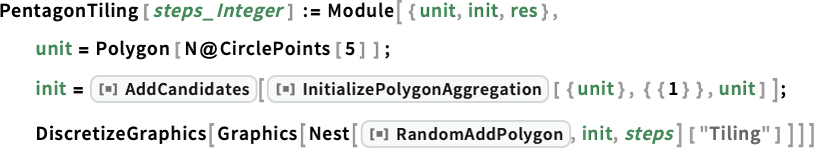
For 20 pentagons I can run this quickly on my machine:
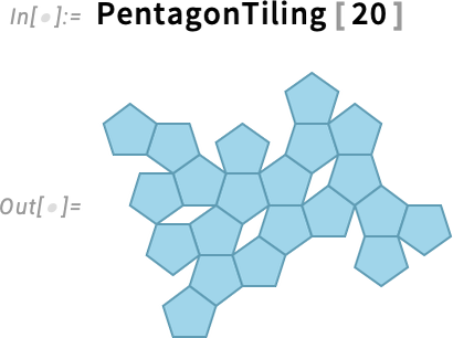
But what about for 500 pentagons? Well, the computational geometry gets difficult and it would take long enough that I wouldn’t want to tie up my own machine doing it. But now there’s another option: use Wolfram Compute Services!
And all I have to do is feed my computation to RemoteBatchSubmit:

Immediately, a job is created (with all necessary dependencies automatically handled). And the job is queued for execution. And then, a couple of minutes later, I get an email:

Not knowing how long it’s going to take, I go off and do something else. But a while later, I’m curious to check how my job is doing. So I click the link in the email and it takes me to a dashboard—and I can see that my job is successfully running:

I go off and do other things. Then, suddenly, I get an email:

It finished! And in the mail is a preview of the result. To get the result as an expression in a Wolfram Language session I just evaluate a line from the email:
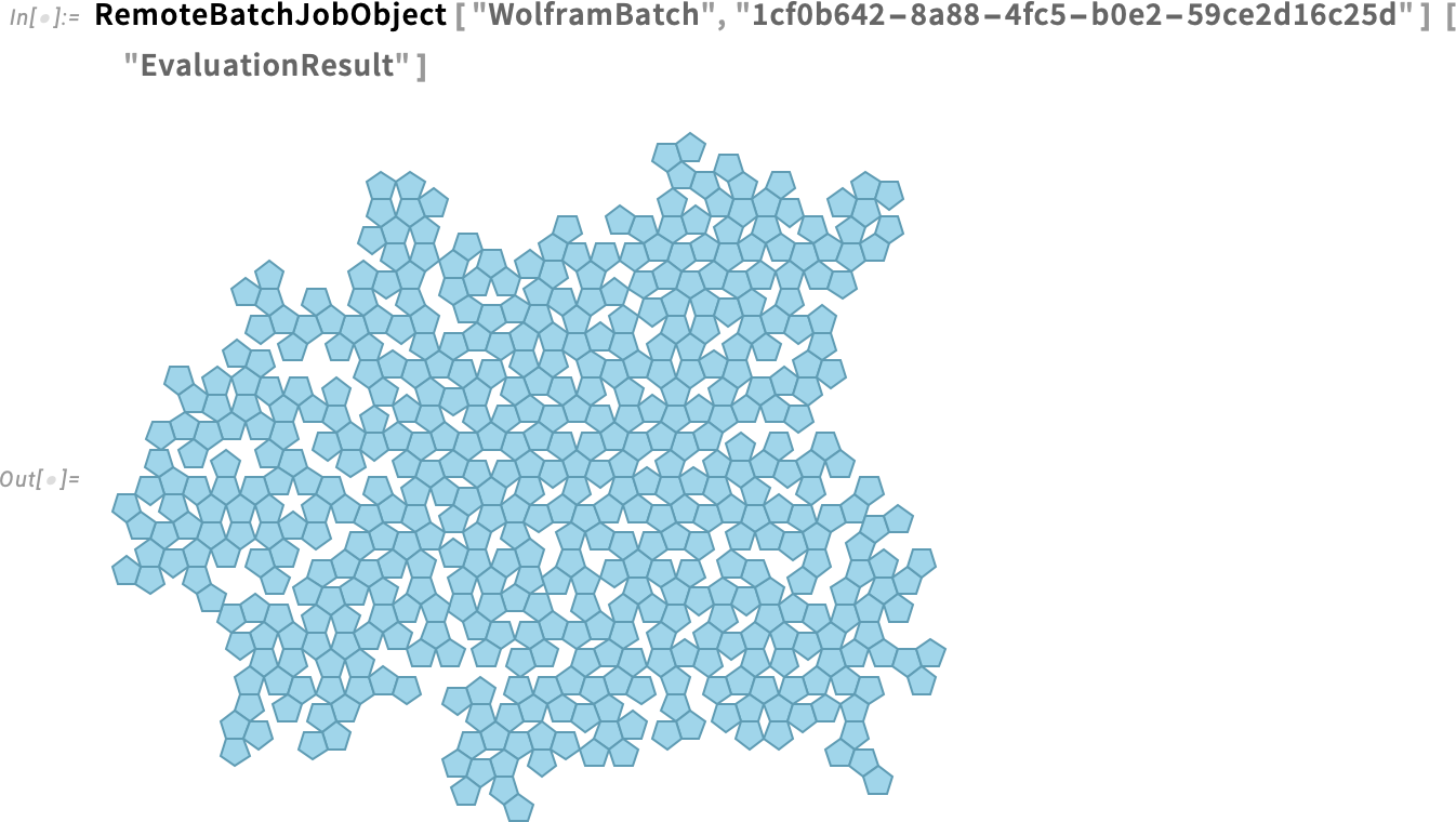
And this is now a computable object that I can work with, say computing areas
or counting holes:
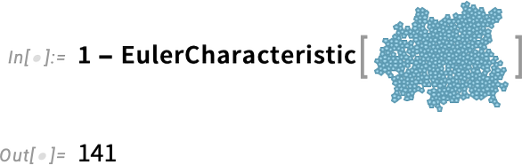
One of the great strengths of Wolfram Compute Services is that it makes it easy to use large-scale parallelism. You want to run your computation in parallel on hundreds of cores? Well, just use Wolfram Compute Services!
Here’s an example that came up in some recent work of mine. I’m searching for a cellular automaton rule that generates a pattern with a “lifetime” of exactly 100 steps. Here I’m testing 10,000 random rules—which takes a couple of seconds, and doesn’t find anything:
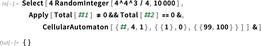
To test 100,000 rules I can use ParallelSelect and run in parallel, say across the 16 cores in my laptop:
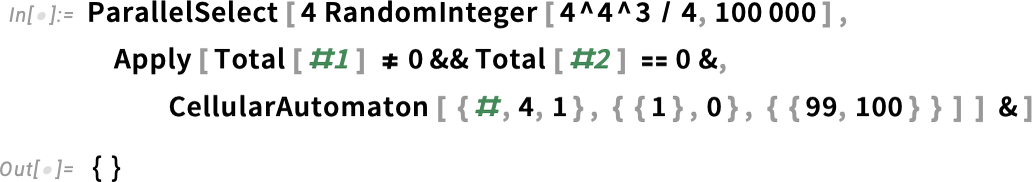
Still nothing. OK, so what about testing 100 million rules? Well, then it’s time for Wolfram Compute Services. The simplest thing to do is just to submit a job requesting a machine with lots of cores (here 192, the maximum currently offered):
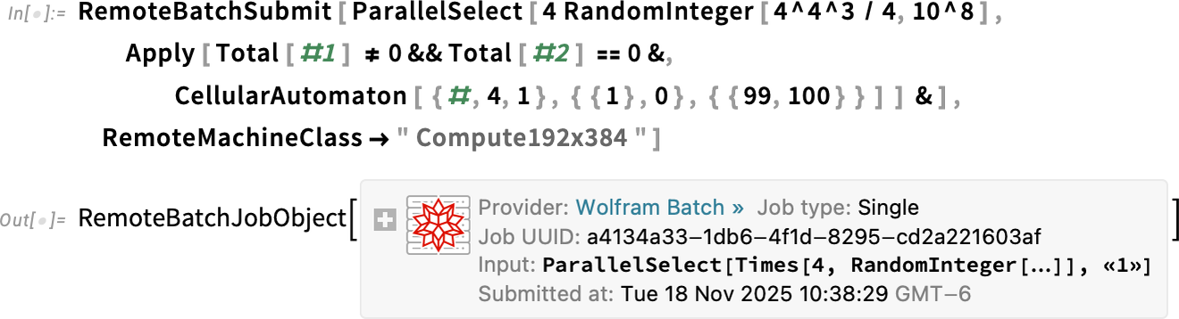
A few minutes later I get mail telling me the job is starting. After a while I check on my job and it’s still running:

I go off and do other things. Then, after a couple of hours I get mail telling me my job is finished. And there’s a preview in the email that shows, yes, it found some things:

I get the result:
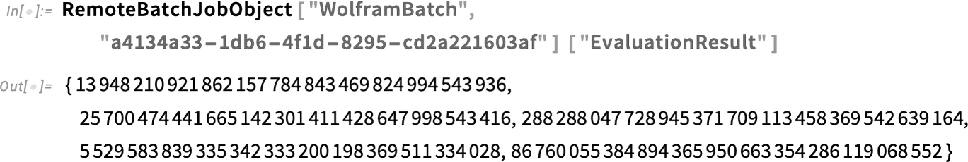
And here they are—rules plucked from the hundred million tests we did in the computational universe:
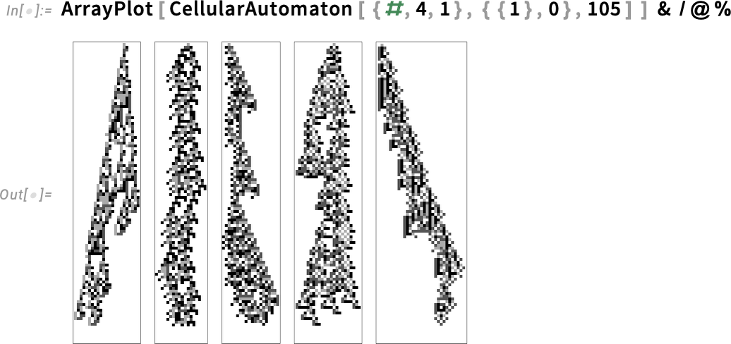
But what if we wanted to get this result in less than a couple of hours? Well, then we’d need even more parallelism. And, actually, Wolfram Compute Services lets us get that too—using RemoteBatchMapSubmit. You can think of RemoteBatchMapSubmit as a souped up analog of ParallelMap—mapping a function across a list of any length, splitting up the necessary computations across cores that can be on different machines, and handling the data and communications involved in a scalable way.
Because RemoteBatchMapSubmit is a “pure Map” we have to rearrange our computation a little—making it run 100,000 cases of selecting from 1000 random instances:
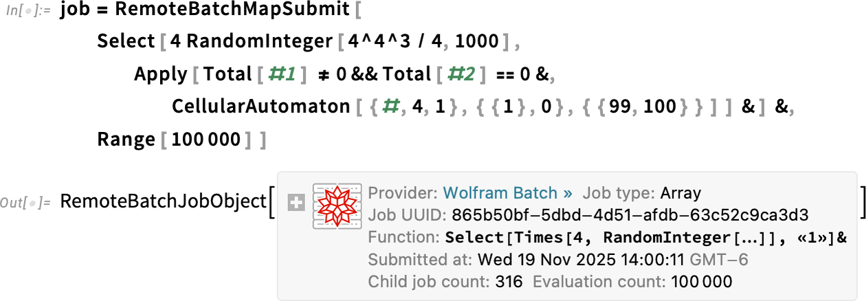
The system decided to distribute my 100,000 cases across 316 separate “child jobs”, here each running on its own core. How is the job doing? I can get a dynamic visualization of what’s happening:
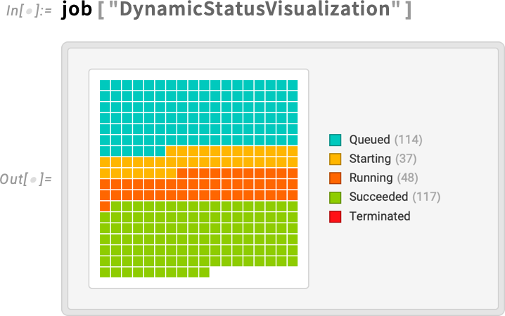
And it doesn’t take many minutes before I’m getting mail that the job is finished:

And, yes, even though I only had to wait for 3 minutes to get this result, the total amount of computer time used—across all the cores—is about 8 hours.
Now I can retrieve all the results, using Catenate to combine all the separate pieces I generated:
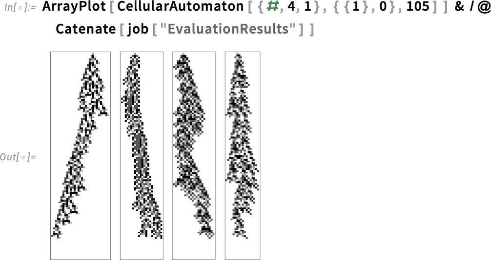
And, yes, if I wanted to spend a little more, I could run a bigger search, increasing the 100,000 to a larger number; RemoteBatchMapSubmit and Wolfram Compute Services would seamlessly scale up.
Like everything around Wolfram Language, Wolfram Compute Services is fully programmable. When you submit a job, there are lots of options you can set. We already saw the option RemoteMachineClass which lets you choose the type of machine to use. Currently the choices range from "Basic1x8" (1 core, 8 GB) through "Basic4x16" (4 cores, 16 GB) to “parallel compute” "Compute192x384" (192 cores, 384 GB) and “large memory” "Memory192x1536" (192 cores, 1536 GB).
Different classes of machine cost different numbers of credits to run. And to make sure things don’t go out of control, you can set the options TimeConstraint (maximum time in seconds) and CreditConstraint (maximum number of credits to use).
Then there’s notification. The default is to send one email when the job is starting, and one when it’s finished. There’s an option RemoteJobName that lets you give a name to each job, so you can more easily tell which job a particular piece of email is about, or where the job is on the web dashboard. (If you don’t give a name to a job, it’ll be referred to by the UUID it’s been assigned.)
The option RemoteJobNotifications lets you say what notifications you want, and how you want to receive them. There can be notifications whenever the status of a job changes, or at specific time intervals, or when specific numbers of credits have been used. You can get notifications either by email, or by text message. And, yes, if you get notified that your job is going to run out of credits, you can always go to the Wolfram Account portal to top up your credits.
There are many properties of jobs that you can query. A central one is "EvaluationResult". But, for example, "EvaluationData" gives you a whole association of related information:
If your job succeeds, it’s pretty likely "EvaluationResult" will be all you need. But if something goes wrong, you can easily drill down to study the details of what happened with the job, for example by looking at "JobLogTabular".
If you want to know all the jobs you’ve initiated, you can always look at the web dashboard, but you can also get symbolic representations of the jobs from:
For any of these job objects, you can ask for properties, and you can for example also apply RemoteBatchJobAbort to abort them.
Once a job has completed, its result will be stored in Wolfram Compute Services—but only for a limited time (currently two weeks). Of course, once you’ve got the result, it’s very easy to store it permanently, for example, by putting it into the Wolfram Cloud using CloudPut[expr]. (If you know you’re going to want to store the result permanently, you can also do the CloudPut right inside your RemoteBatchSubmit.)
Talking about programmatic uses of Wolfram Compute Services, here’s another example: let’s say you want to generate a compute-intensive report once a week. Well, then you can put together several very high-level Wolfram Language functions to deploy a scheduled task that will run in the Wolfram Cloud to initiate jobs for Wolfram Compute Services:
And, yes, you can initiate a Wolfram Compute Services job from any Wolfram Language system, whether on the desktop or in the cloud.
Wolfram Compute Services is going to be very useful to many people. But actually it’s just part of a much larger constellation of capabilities aimed at broadening the ways Wolfram Language can be used.
Mathematica and the Wolfram Language started—back in 1988—as desktop systems. But even at the very beginning, there was a capability to run the notebook front end on one machine, and then have a “remote kernel” on another machine. (In those days we supported, among other things, communication via phone line!) In 2008 we introduced built-in parallel computation capabilities like ParallelMap and ParallelTable. Then in 2014 we introduced the Wolfram Cloud—both replicating the core functionality of Wolfram Notebooks on the web, and providing services such as instant APIs and scheduled tasks. Soon thereafter, we introduced the Enterprise Private Cloud—a private version of Wolfram Cloud. In 2021 we introduced Wolfram Application Server to deliver high-performance APIs (and it’s what we now use, for example, for Wolfram|Alpha). Along the way, in 2019, we introduced Wolfram Engine as a streamlined server and command-line deployment of Wolfram Language. Around Wolfram Engine we built WSTPServer to serve Wolfram Engine capabilities on local networks, and we introduced WolframScript to provide a deployment-agnostic way to run command-line-style Wolfram Language code. In 2020 we then introduced the first version of RemoteBatchSubmit, to be used with cloud services such as AWS and Azure. But unlike with Wolfram Compute Services, this required “do it yourself” provisioning and licensing with the cloud services. And, finally, now, that’s what we’ve automated in Wolfram Compute Services.
OK, so what’s next? An important direction is the forthcoming Wolfram HPCKit—for organizations with their own large-scale compute facilities to set up their own back ends to RemoteBatchSubmit, etc. RemoteBatchSubmit is built in a very general way, that allows different “batch computation providers” to be plugged in. Wolfram Compute Services is initially set up to support just one standard batch computation provider: "WolframBatch". HPCKit will allow organizations to configure their own compute facilities (often with our help) to serve as batch computation providers, extending the streamlined experience of Wolfram Compute Services to on-premise or organizational compute facilities, and automating what is often a rather fiddly job process of submission (which, I must say, personally reminds me a lot of the mainframe job control systems I used in the 1970s).
Wolfram Compute Services is currently set up purely as a batch computation environment. But within the Wolfram System, we have the capability to support synchronous remote computation, and we’re planning to extend Wolfram Compute Services to offer this—allowing one, for example, to seamlessly run a remote kernel on a large or exotic remote machine.
But this is for the future. Today we’re launching the first version of Wolfram Compute Services. Which makes “supercomputer power” immediately available for any Wolfram Language computation. I think it’s going to be very useful to a broad range of users of Wolfram Language. I know I’m going to be using it a lot.